1. Introduction

In this section, I’ll lay out why decarbonization of the US power grid matters, provide a high-level overview of the current situation and economic trends, and then address why such a proper solution to the problem has high complexity.

1.1 Doom and Gloom: Why Reaching Zero Carbon Matters

In October 2018, the Intergovernmental Panel on Climate Change (IPCC) published a special report on the impact of a global average temperature rise of 1.5°C over pre-industrial levels [i]. The message wasn’t pretty. It mentioned “hot extremes in most inhabited regions”, with an increase of the extreme temperatures in the mid-latitudes by about 5 degrees Fahrenheit. It discussed “increases in frequency, intensity, and/or amount of heavy precipitation in several regions” alongside “the probability of drought and precipitation deficits in some regions”. It predicted that sea levels could rise by somewhere just under a foot to over two-and-a-half feet by 2100 (with every four inches representing 10 million people exposed to related risks). The report discussed how 1.5°C represented the possibility of a climate “tipping point” of sorts – beyond 1.5°C, dangerous feedback loops would start to enter the picture [1]. Should the ice sheets in Antarctica or Greenland become unstable, it could result sea levels rising several yards over hundreds to thousands of years. The report touched on ocean acidification leading to species loss and extinction (and amplifying other effects). All of the doom-and-gloom contained in a world 1.5°C hotter than pre-1750 was succinctly summarized by the report with “[c]limate-related risks to health, livelihoods, food security, water supply, human security, and economic growth are projected to increase with global warming of 1.5°C”.

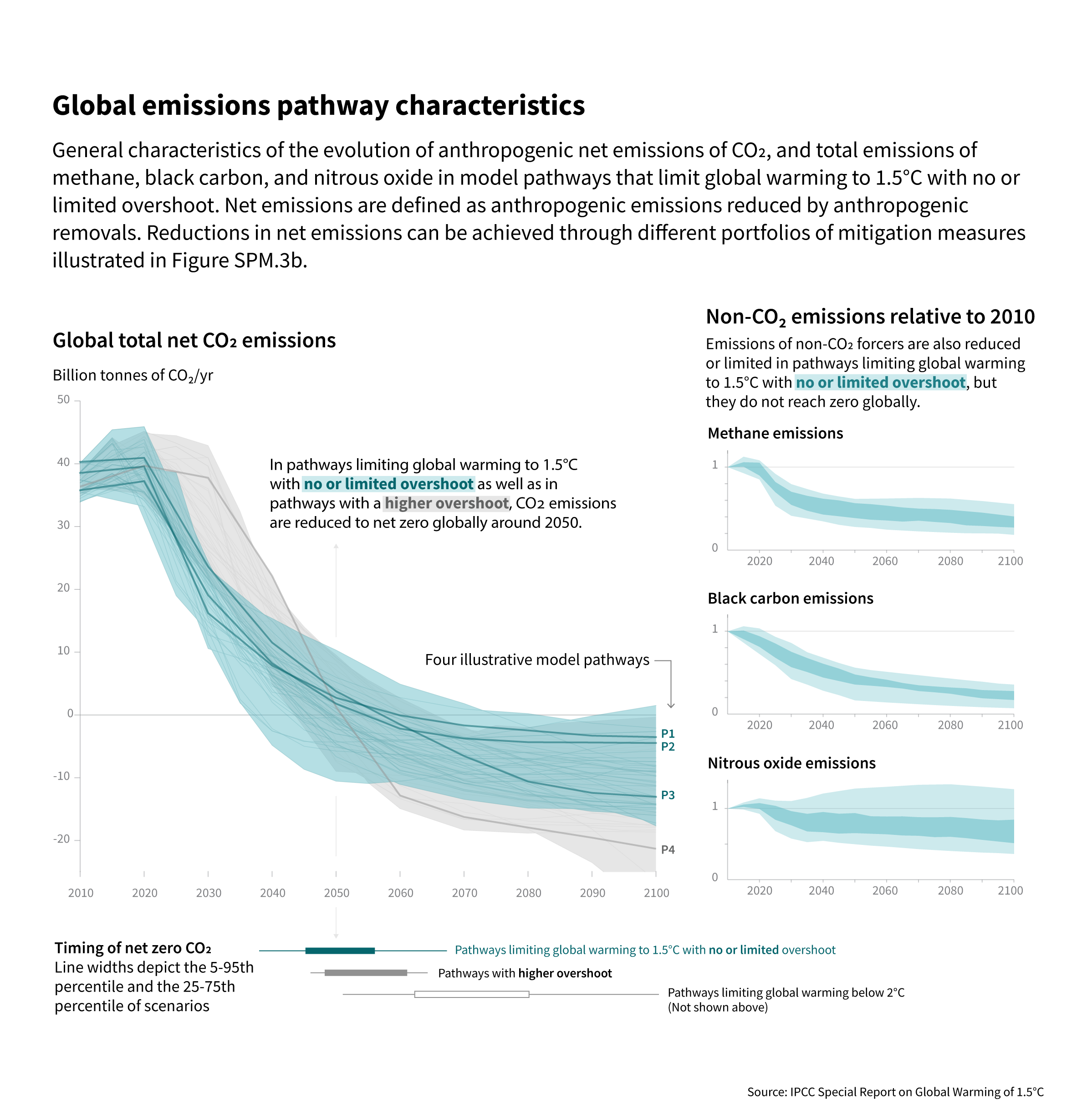
As bad as the 1.5 degree threshold may sound, it’s a almost a goal at this point. The world is likely to hit the 1.5 degrees warmer sometime between 2030 and 2052, and we’re already at 1 degree of temperature increase. Achieving a 1.5 degree path with a limited amount of “overshoot” (temporarily crossing the 1.5 degree line before retreating back) would require reducing our global emissions by 40-60% between 2010 and 2030, and hitting global net-zero emissions sometime around 2050 (give or take 5 years). All of this “would require rapid and far-reaching transitions in energy, land, urban and infrastructure (including transport and buildings... unprecedented in terms of scale”. For energy and electricity use specifically, the report notes a need to both electrify energy end use faster (i.e. use electricity for more processes where we currently use fossil fuels), cut back substantially on coal and natural gas use for electricity generation, and implement more carbon capture and storage (CCS). There is a small nugget of hope for this transition, however: the IPCC notes that “…political, economic, social and technical feasibility of solar energy, wind energy and electricity storage technologies have substantially improved over the past few years… These improvements signal a potential system transition in electricity generation.”

Figure 1: Model Pathways to 1.5 degrees of Warming [ii]

Which brings us to the US. If a global clean energy and electricity transition is to have any shot at success, it will have to include the US. In 2019, the US produced about one-seventh of global energy-related emissions [iii]. In 2018, the US emitted 6,677 million metric tons of CO2 equivalent [2], and the electricity sector accounted for 27% of these emissions [iv]: roughly 1,800 million metric tons of CO2 equivalent [3][v], or roughly the equivalent from burning 10 million railcars’ worth of coal [4]. While overall emissions from the US power grid have fallen by 27% from their peak in 2007 [vi], estimates for the social cost of pollution related to US electricity production (i.e. the costs not directly paid by emitters, perhaps in the form of reduced air quality or premature deaths) just in 2011 are $147B [5]. We’re already paying the cost for pollution from the electricity sector; the damaging effects aren’t just in the future.

1.2 Achieving a Zero Carbon Economy Requires Electrifying (Perhaps) Everything, and Cleaning up the Electricity Sector

The electricity sector in particular is presented with a unique demand on the road to net-zero: because it enables other industries and sectors to decarbonize, it must more rapidly decarbonize in order to not delay the overall decarbonization path. In other words, the electricity sector acts as a sort of bottleneck to the decarbonization of other sectors.

It helps to understand the nomenclature of the different scopes of emissions. Scope 1 emissions can be directly attributed to an organization, business, or sector: this refers to “the direct burning of fossil fuels in generators, facilities, and vehicles” [vii]. Scope 2 emissions refers to purchased energy that wasn’t directly generated, such as electricity, and Scope 3 emissions refers to emissions further up-and-down the value chain. While much more complex than Scope 1 and Scope 2, it can be loosely thought of as including the emissions associated with suppliers and customers. As a household-level example, Scope 1 emissions come from the gasoline we fuel our cars with, the generators we run during a power outage, or the natural gas we use for cooking. Scope 2 emissions are the emissions incurred to produce the electricity we used. Scope 3 emissions come from the products we use and make in our home – paper towels, beef pot roast, our clothing. The beef pot roast we have for dinner wouldn’t have been consumed without us; therefore we’re responsible for the emissions.

Figure 2: Three Scopes of Emissions, for a Federal Agency [viii]

For many industries with currently high Scope 1 emissions, the path to decarbonization relies on shifting Scope 1 emissions to Scope 2 emissions, and relying on clean electricity to negate Scope 2 emissions. Transportation represents a fairly high-profile example: in 2018, transportation accounted for 28% of US greenhouse gas emissions, over half of which was due to passenger cars and trucks [ix]. While the barriers to electrification may be high for airplanes, ships, or Class 8 long-haul trucks towing tens of thousands of pounds, barriers to electrifying passenger vehicles are much lower, and electric cars have being steadily increasing adoption rates across the world. Such electrification can be driven by shifts in consumer perceptions on economics, performance, and practicality [x]. Replacing a gasoline-powered family vehicle with an electric one shifts emissions from Scope 1 to Scope 2, and as the power grid relies more on zero-carbon sources, the overall emissions impact of an electric vehicle falls further.

For heavy industry, a similar shift will have to occur. Industry produced 22% of 2018 US emissions (not including Scope 2, which the EPA attributed to the earlier 28%) [xi]. Most of the 22% came from Scope 1 emissions, though a similar strategy of electrifying equipment to shift Scope 1 emissions to Scope 2 emissions presents a key opportunity for driving sector decarbonization. If heavy industry shifts toward more electric equipment, then that equipment’s carbon footprint is essentially linked to that of the power grid. Clean up the power grid, and the equipment is also cleaned up automatically [6]. For heavy industry, electrification also represents a potential economic benefit, with some use cases benefitting from higher performance and lower total cost of ownership [7][xii].

For transportation, industry, and other sectors, shifting Scope 1 emissions to Scope 2 emissions through electrification has two benefits for decarbonization: (1) electrification tends to bring with it increased energy efficiency, which immediately lowers overall emissions, and (2) the amount of carbon emitted per unit of energy consumed isn’t fixed and has steadily decreased in the US over the past 15 years [8][xiii]. Indeed, Sterchele et al. find that “the more ambitious the climate protection targets are, the faster the required transition from a fossil fuel-based demand to a demand dominated by electric technologies, i.e., the consumption sectors get progressively electrified” [9][xiv].

Estimates of the overall energy that we can save by electrifying everything are around the 45% mark [xv]. In other words, transitioning current fossil-fuel-based demand to electricity would reduce the total amount of energy that we consume in the first place, mostly due to higher the efficiency inherent to electrification (e.g. electric cars are more efficient than gasoline cars, on a miles-per-unit-energy basis) and to the lack of energy spent in the fossil fuel supply chain – extraction, refining, transportation, etc.

However, a reduction in energy isn’t a reduction in electricity. The upshot is that we need to vastly scale the power grid if we are to increasingly electrify more and more sources of energy demand. Furthermore, to achieve real progress toward zero-carbon, we’d have to not only transition existing electricity generation sources to zero-carbon ones, but also ensure that new capacity that’s built is also zero-carbon.

1.3 Where we are Now

The United States encompasses a large landmass with incredibly varied terrain. As a result, it may not be too surprising that there is no one “national grid”, such as the one the United Kingdom built to service the entire island of Great Britain – geography represents a fundamental barrier to this task. Nevertheless, many regions and smaller grids connected together into three “interconnects”, which serve as larger grids themselves. Thus, the “US grid” can be thought of as three grids: (1) the Western Interconnect, which services the area west of the Rockies, (2) the Texas Interconnect, which serves the majority of Texas, and (3) the Eastern Interconnect, which services the area east of the Rockies (except Texas) [xvi]. Interconnections are themselves aggregations of smaller networks of generators and transmission lines. They help provide resiliency and stability in a system where, at any given microsecond, power generation must match up with power consumption [10]. If a power line or a generator were to fail, another transmission line or generator could essentially pick up the slack while repairs are made. However, these grids are mostly separate – there’s very little capacity to share electricity from any of the interconnects to any other. Thus, a power plant failure in Texas couldn’t be overcome with extra capacity from a plant in New Mexico, though an outage in Charlotte could be indirectly aided with capacity from Chicago. To give a sense of scale, in 2016 peak demand for the Western Interconnect was around 140 GW, 70 GW for the Texas Interconnect, and 450 GW for the Eastern Interconnect [xvii] (see Appendix A1 for a discussion of power vs. energy and common units). To avoid backouts, each grid needs to have enough electricity generating capacity to cover these peak demand scenarios.

Figure 3: Interconnections of the US Power Grid [xviii]

On the generation front, there’s roughly 1,100 GW of summer utility-scale capacity across the country [xix] (energy demand peaks in most of the US occurs in the summer, so it’s important to measure how much capacity is available then, and utility-scale ignores smaller-scale generation sources like rooftop solar). 67% of summer capacity comes from fossil fuels, nuclear provides about 9% of capacity, and 13% of capacity comes from wind and solar. Power isn’t the same as energy, however, so there isn’t a one-to-one relationship between sources of capacity (power) and sources of electricity (energy). For example, nuclear power plants tend to constantly be producing electricity, whereas solar panels can’t produce 100% of possible power at every instant throughout the day (due to the natural cycle of the sun, along with weather patterns). A plant’s capacity factor defines how much electricity a plant produces as a percentage of how much that plant could produce, if it were running at nonstop full capacity [xx]. For all of 2019, nuclear power plants had a capacity factor well over 90%, solar had a capacity factor around 25%, and natural gas plants averaged 57% [xxi]. Thus, we’d expect nuclear to produce more electricity than its share of generating capacity, and solar to produce less.

From the energy perspective, the US produced just over 4,100 TWh of electricity in 2019. Fossil fuels accounted for 63% of the electricity produced, nuclear provided about 20%, and renewables made up the remaining 18% [11]. Breaking apart the renewables category, 7% (of the total electricity production, not of the renewables share) comes from wind, another 7% from hydropower, and solar takes up 2%. Biomass, geothermal, and other sources round out the remainder [xxii]. While the snapshot doesn’t sound encouraging, the trends certainly can be.

Figure 4: US Electricity Production, 2000-2020 [xxiii]

Wind and solar electricity production have grown at an exponential rate over the past decade, driven by increasingly improving economics. In 2000, wind produced 5.6 TWh of electricity, and grew to 17.8 TWh in 2005 (3.2x in 5 years), 94.7 TWh in 2010 (5.3x in 5 years), 190.7 TWh in 2015 (2x in 5 years), and over 300 by 2019 (1.6x in 4 years). From a capacity standpoint, wind capacity grew from 2 GW in 2000 to 104 GW in 2019. Solar is practically out of the picture until 2007, when growth began – in 2007, solar produced 0.6 TWh of electricity. Four years later in 2011, solar had tripled in production to 1.8 TWh. In 2015, solar accounted for 24.9 TWh (13.8x in 4 years), and in 2019 solar generated 72.2 TWh of electricity (2.9x in 4 years) [xxiv]. The slowdown in growth on a multiplicative-factor basis is mostly due to the near-irrelevance of wind and solar electricity at the turn of the century, though it hides the fact that the two are growing on an absolute basis at breakneck speed. Solar’s capacity has grown from less than a GW to 37 GW in 2019 [xxv]. These capacity expansions are the result of large investments in building out renewable electricity capacity – in the 2010s, wind investment in the US alone totaled $165B, while solar investment was even higher at $211B [xxvi]. This incredible growth and investment contrasts against the stagnation of hydropower and nuclear electricity, which have had stable shares of electricity generation and much less investment.

On the fossil-fuels side of electricity, there’s been a massive shift away from coal and toward the use at natural gas. Coal once dominated the US electricity sector, with an absolute annual peak of 2,016 TWh produced during 2007. This represented 48.5% of all US electricity production that year. In 2019, coal produced 966 TWh of electricity, or 23.5% of US electricity production that year [xxvii]. The past 12 years have seen coal’s share of the electricity production shrink to half of what it was previously, despite only a ~1% drop in total electricity consumption. It’s immediately worth noting the contrast in scale to solar and wind. The drop in electricity production from coal was 5.5x the amount of wind energy produced in 2019, and almost 15x the amount of solar energy produced in 2019. Despite rapid growth in renewables, the scale wasn’t yet there for renewables to displace coal at a national scale. That came from natural gas. In 2007, it accounted for 897 TWh of electricity production; by 2019 it represented 1,582 TWh, (making up for 65% of coal’s decline). Today, natural gas accounts for 38.5% of US electricity production, making it the dominant source of electricity.

The rise of natural gas is largely a function of lower prices, both for construction and operation. After a peak in 2008 at $9.26/1000 cubic feet, a US fracking boom in shale gas led to prices for natural gas for electricity producers falling steeply [12]. Prices dropped nearly 50% the next year and have continued a steady downward trend since then. In 2019, the price for natural gas reached below $3 [xxviii]. Natural gas combined cycle plants also benefitted from low capital costs, high efficiencies, and fast construction times [xxix]. Coal-fired power plants are no longer competitive, and the last new coal plant to be built within the US was in 2015 [xxx].

For the most part, economics is what drove the shift in electricity generation sources. Electricity is a commodity; neither your toaster nor the power lines carrying power across the country can tell the difference between electricity generated from a solar panel or a coal plant. As a result, electricity functionally has the same selling price, regardless of source [13]. Profits, therefore, almost entirely depend on cost, and no metric captures cost of electricity better than the Levelized Cost of Electricity (LCOE). Windmills and solar panels are different from a natural gas or nuclear power plants since they have functionally zero marginal costs. Unlike nuclear or natural gas power plants that must keep buying fuel, once a windmill or solar panel is built and the upfront cost is paid, there’s little cost to the owner beyond general maintenance. The LCOE essentially represents the total costs paid for a generator (including interest, tax credits, maintenance, fuel, etc.) divided by the amount of electricity produced [xxxi].

From this LCOE perspective, renewables are the cheapest [14] source of electricity available in the US. The EIA estimates that solar’s LCOE is around $33/MWh, before tax incentives, for new plants entering service in 2025, compared to $34/MWh for onshore wind, $37/MWh for natural gas, and $40/MWh for hydroelectric plants [xxxii]. Furthermore, both wind and solar have been getting steadily cheaper over time as production and installations have grown [15] – from 2015 to 2020, the cost of wind electricity fell 5% annually, while the cost of solar electricity fell 11% annually [xxxiii], as shown in the graph below:

Figure 5: LCOE of Wind and Solar Electricity, 2009 – 2020 [xxxiv]

That cost advantage means that solar and wind should be built out at an increasingly rapid rate – the explosive growth discussed earlier is only the early stages of wind and solar electricity being competitive in certain regions. As solar and wind become more competitive in more regions, an acceleration in deployment is likely. In 2019, wind, solar, and natural gas accounted for 46%, 18%, and 34% (respectively) of planned capacity additions during the year, while coal, natural gas, and nuclear accounted for 53%, 27%, and 18% (respectively) of planned capacity retirements [xxxv]. Cheaper sources are winning out, at the expense of older, more expensive ones.

Figure 6: Grid Additions and Retirements: From Coal to Renewables and Natural Gas [xxxvi]

1.4 How far do we need to go to get to a 100% Zero-carbon Power Grid?

One of President Biden’s campaign targets was to achieve a zero-carbon power grid by 2035 [xxxvii]. That’s an ambitious goal, one that will require considerable effort and resources to be even potentially feasible. Different forecasts produce different estimates of how much capacity the power grid will need in the future. These numbers vary due to differing assumptions in energy efficiency, the speed of electrification of other sectors, and the presence of net-zero policies. Predicting the future is hard – especially when that future is 30 years out – but these estimates can provide a helpful guide for how much capacity the grid will need.

The National Renewable Energy Laboratory (NREL) published the Electrification Futures Study in 2018 indicating ~4,700 TWh of electricity demand in 2050 under a business-as-usual approach, ~5,650 TWh under a “Medium” scenario (which involves some easily accomplished electrification), and ~6,500 TWh under a “High” scenario (where a more aggressive electrification approach is taken). The same study estimated that national peak demand could reach 838, 997, and 1114 GW under the business-as-usual, Medium, and High scenarios respectively [16][xxxviii]. The “High” scenario implies a kind of transformative growth in electrification (though not necessarily broad enough for a net-zero society), and the numbers imply a ~70% increase in capacity for the power grid (both in terms of energy and power).

Another estimate by Jacobson et al. [xxxix] uses a first-principles approach to determining a “goal” grid size: first, they forecast total energy use in 2050 by country (using data from the IEA and EIA), and then examine the effect that 100% electrification would have. After obtaining a 45% estimate on overall efficiency improvements [17], they estimate that total, end-user electricity use (i.e. the amount of electricity that actually reaches homes, businesses, and industry) is ~11,300 TWh [18]. Assuming a 5% transmission loss [xl], that means the US would need to produce ~11,900 TWh [19] of electricity each year. For comparison, in 2019, the US delivered [20] ~3,700 TWh of electricity to consumers. Therefore, we’d need to grow the power grid by roughly 200% [21] in order to cope with such a transition – and to make the grid zero-carbon, all existing and all new generation would need to come from nuclear, wind, solar, and other zero-carbon sources. That 45% is a critical assumption – if the overall savings are a more conservative 35%, we’d need to bolster the size of the grid by about 260% [22] to support a net-zero transition.

Regardless of whether the NREL study or the Jacobson et al. study turns out to be more accurate, we’ll need to vastly expand renewable electricity production. Considering that zero-carbon sources didn’t even produce 40% of the electricity the US used in 2019, transitioning to a zero-carbon grid within 15 years is quite the moonshot [23]. It isn’t a straightforward solution – merely scaling up the existing power grid by adding more wind and solar capacity won’t cut it.

1.5 Reliability Concerns from Variable Renewable Energy’s Intermittency and Seasonality

Intermittency and seasonality are two crucial issues with wind and solar that create reliability issues, on different ends of time scales: intermittency raises a minute-to-minute or day-to-day issue, while seasonality represents a more annual problem.

Wind and solar belong to a class of electricity sources called Variable Renewable Energy (VRE) – essentially, the output from these sources of electricity is hard to reliably predict. We can estimate, on average, the amount of electricity that a wind turbine or solar panel will produce in a specific location (given historical weather data, for example). However, there’s little control we get over the output on a second-by-second level. Generators fueled by nuclear or fossil fuel sources are controllable; operators can turn them on or off as they see fit. A wind turbine or solar panel, however, may produce different amounts of electricity from one minute to the next (e.g. due to cloud cover) or one day to the next (e.g. due to a weather system passing through the area, creating cloudy conditions for a few consecutive days), which creates an issue for grid operators. For example, a windy/sunny day may be followed by a calm/overcast one [24]. At any given instant, supply must match demand, which is difficult to accomplish given the high intermittency from wind and solar if these sources account for a large percentage of the grid’s generation capacity.

A slightly different issue that nevertheless manifests itself on a similar scale is a phenomenon referred to as a “duck curve” [xli]. In an area with sizeable market penetration of rooftop commercial/residential solar (which is “behind-the-meter”, in that electricity generation occurs at the consumer site and thus affects how much power the user draws from the grid in the first place), the amount of power demanded drops during the daytime as solar panels begin producing energy. At night, however, electricity use ramps up quickly: both due to solar panels no longer producing behind-the-meter power, and also as “gross” [25] power demand rises (e.g. when people come home from work and begin cooking and running the laundry). This in turn creates a need for higher grid infrastructure flexibility, as generators need to be able to shut down during the day and restart to meet the evening demand. Intermittency issues can be mitigated by deploying energy storage systems and spreading generation across a wider variety of geographies [26][xlii].

Figure 7: The Duck Curve [xliii]

Figure 8: CA Solar Electricity Production by Hour [xliv]

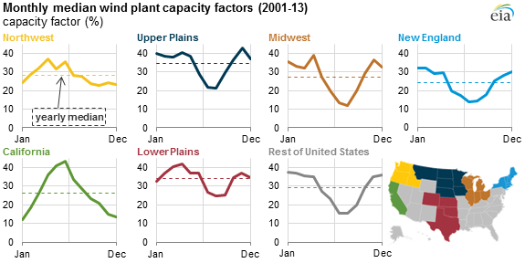
At a larger scale, seasonality refers to patterns in electricity production over the course of a year. Solar panels produce may more electricity in the summer (when days are longer) than in the winter [xlv]; wind turbines tend to produce more electricity during the spring and less during the back half of the summer – in California, for example, wind power has an average capacity factor of over 40% during the late spring months and below 20% during the winter [xlvi]. The pacific northwest region of the US has less variation in wind seasonality, but capacity factors dip below 25% from September through January, and reaches around 35% from March through June. For solar, the US produced about 10 TWh of solar electricity in July of 2020, but only just above 5 TWh in December of 2020 [xlvii]. A true zero-carbon grid can’t just have enough capacity for spring days when wind and solar electricity generation is plentiful and overall electricity demand is low; reliability requires the grid being able to match supply with demand even during periods of cloudy and cold/hot of days (when electricity usage peaks to keep homes warm/cool and when generation is weakest). Seasonality can be mitigated with capacity overbuilding – though due to lower utilization of the overbuilt capacity, such generation is inherently less profitable.

Figure 9: Wind Capacity Factors Vary by Region and Season [xlviii]

The rest of this thesis attempts to answer the question of how we get from eighteen hundred (million metric tons of annual emissions) to zero, given the hurdles that we know of (especially seasonality and intermittency). A variety of proposed solutions exist, each of them tackling one piece of the puzzle – reliability, new generation capacity, energy storage, etc. I’ll discuss those solutions, explore some scenarios that combine those solutions, and then discuss some policies that could be enacted to accelerate the transition to a bigger, better power grid. However, it’s worth noting that specifics are difficult to come by – estimating exactly how much of any one solution we’ll need is foolhardy and pointless – we can’t really know exactly how much energy storage we’ll need, or how much excess capacity we’ll need to build. In the end, getting to a fully decarbonized power grid is going to require an all-of-the-above approach, as frustratingly nebulous as that may be.

---

[1] https://www.mckinsey.com/business-functions/sustainability/our-insights/climate-math-what-it-takes-to-limit-warming-to-1-point-5-degrees-c mentions a few of these: “If we lose our forests, which would happen at higher-climate-change levels, that will cause more global warming… similarly, losing ice cover warms the Earth. And so the global warming that is leading to the ice loss could then drive further global warming.”

[2] This means that other emitted gases (e.g. methane, nitrous oxide) were converted to CO2 emissions using the 100-year Global Warming Potential. Some gases also have different rates of affecting the climate: for example, methane warms the atmosphere much more than carbon dioxide does over 20 years than it does over a 100 year timescale. More information is available at https://www.epa.gov/ghgemissions/understanding-global-warming-potentials

[3] For some perspective, annual global emissions from all sources are roughly around 50 gigatons (or 50,000 million metric tons) in CO2e – this entire paper is focused on roughly three-and-change percent of global annual emissions.

[4] A railcar holds about 200,000 pounds of coal. Readers interested in other conversions for more intuitive units can find various conversion factors at https://www.epa.gov/energy/greenhouse-gases-equivalencies-calculator-calculations-and-references.

[5] I use a Value of a Statistical Life of $8.3 million, and inflation adjust the author’s estimate from 2011 to 2020 using https://www.bls.gov/data/inflation_calculator.htm. See Appendix A2 for a more thorough discussion on the costs of externalities associated with electricity production.

[6] This is ignoring the emissions associated with production of that equipment, which aren’t necessarily zeroed out through a zero-carbon power grid.

[7] It’s worth noting that not all industrial processes are currently at a stage that’s ripe for electrification; some, such as the manufacturing of cement or steel, are going to be more tricky to decarbonize.

[8] In 2005, the US produced 606 grams of CO2-equivalent emissions for each kWh of electricity generated. In 2018 (the most recent year for which I could find all the necessary data), that figure dropped to 431 g CO2e / kWh – a 29% drop. This hasn’t just been driven by renewables – it’s also due to all forms of generation becoming more efficient, and coal-fired power plants being replaced natural-gas ones.

[9] I’d recommend the NREL Electrification Futures Study (https://www.nrel.gov/docs/fy21osti/72330.pdf) to the reader interested in understanding how different levels of electrification affect the build-out of the US power grid. 

[10] While energy storage is growing in size, the amount of energy that we could store in total currently represents very little of the electricity generated or consumed on any given day. This is the fundamental driver behind the need to perfectly balance supply and demand. Once energy storage capacities are far higher, it may be possible to overproduce electricity during one part of the day, and use the surplus to satisfy demand during a period of time when production may be lower. More on this later.

[11] These don’t add up to 100% due to rounding.

[12] You can see the explosion in production with the charts at https://www.eia.gov/energyexplained/natural-gas/where-our-natural-gas-comes-from.php.

[13] There are extra revenue opportunities in some markets for carbon-free power, though the general point holds true: there’s one electricity market settlement price.

[14] Since fuel costs and electricity produced can vary from place to place (e.g. solar panels will produce more energy in Arizona than in New England), accurate LCOE estimates can only be assigned to a particular technology in a particular region. Therefore, LCOE estimates are usually given either as a range (best-case to worst-case) or a capacity-weight average (the average LCOE, weighted by the size of the generators)

[15] Swanson’s Law is the name of this phenomenon for solar, though the more generalized version is called Wright’s Law, which basically relates a doubling in production to a percentage decline in cost (https://ark-invest.com/wrights-law/). Wright’s Law has been applied to multiple industries, though “experience curves” and “cost curves” are frequently applied to modeling the cost of renewable energy production and battery production.

[16] The “Medium scenario” involves electrification in transportation, heat pumps, and some industrial settings, and the “High scenario” involves a “transformational change” in the scope of electricity usage.

[17] This is the 45% figure mentioned earlier toward the end of Section 1.2. The 45.3% reduction comes from three sources: (1) 27.6% from higher efficiency in electrified processes (e.g. electric transportation, heat pumps for heating, etc.), (2) 10.9% from eliminating fossil-fuel infrastructure (e.g. procurement, transport, refining, etc.), and (3) 6.8% from further energy efficiency due to public policy. I later use 35% in what-if analysis as a more conservative reduction estimate by reducing the first two factors by 10% and eliminating the third altogether.

[18] Regrettably, Jacobson et al. publish energy use as an average annual load. This is obviously confusing, as the listed units are in GW, rather than actual units of energy, like GW-years. We convert their estimate of 1291.4 GWy to TWh as follows: 1291.4 GWy x (33.434 Quads / GWy) x (293.07 TWh / Quad) = 11,320. TWh

[19] 11320 TWh / 0.95 = 11916 TWh

[20] This figure is after transmission & distribution (T&D) losses on the power grid – there’s some level of inefficiency in transporting electricity on power lines; this figure accounts for that. We convert the source’s Quads figure to TWh as follows: 12.7 Quads x (293.07 TWh / Quad) = 3,722 TWh.

[21] (11320 – 3722) / 3722 = 204.1%

[22] With only 35% efficiency savings, the US grid would need to deliver (11320 / 0.55) x 0.65 = 13,378 Quads of electricity. (13378 – 3722) / 3722 = 259.4%

[23] It’s worth noting that while this may be a moonshot, it’s only one of many needed. Cleaning up and scaling the US electricity sector is, metaphorically speaking, a drop in the bucket of fighting climate change, since similar transitions will be necessary across the globe. As hinted at earlier, fighting climate change not only requires a change in the way we use energy (the electrification of buildings, industry, and transport) but also a revamp of how we use land (e.g. the agricultural and forestry sector) – exploring any of these topics could merit their own theses.

[24] https://www.cmu.edu/ceic/assets/docs/publications/working-papers/ceic-07-12.pdf provides actual data showing variation in energy production across multiple days at the resolution of minutes to seconds.

[25] “Net” load refers to the overall power consumption (load) at a given moment, after subtracting out VRE production (i.e. wind and solar). I use the term “gross” load to refer to the amount of load before subtracting out VRE production.

[26] While weather is correlated from one location to the next, that correlation decreases as the locations grow farther apart. Summing up all of the wind or solar resources on a grid across a variety of geographies may increase a grid operator’s ability to forecast electricity generation from those units, which in turns assists with balancing supply and demand. This might seem to contradict the earlier notion that a larger percentage of wind and solar makes it harder to balance the grid; even though solar and wind electricity generation may be more predictable, there’s still a larger percentage of the grid’s power that’s subject to variability: while solar power may be plentiful one day, it may be lower the next, though the grid must be able to reliably provide power under prolonger scenarios of cloudy weather.

---

Sources

[i] https://www.ipcc.ch/sr15/chapter/spm/

[ii] https://www.ipcc.ch/site/assets/uploads/sites/2/2019/02/SPM3a.png

[iii] https://www.iea.org/articles/global-co2-emissions-in-2019

[iv] https://www.epa.gov/ghgemissions/sources-greenhouse-gas-emissions

[v] https://cfpub.epa.gov/ghgdata/inventoryexplorer/#electricitygeneration/allgas/source/current

[vi] https://cfpub.epa.gov/ghgdata/inventoryexplorer/

[vii] https://www.bloomberg.com/news/articles/2020-12-08/lawyers-and-publicists-need-their-own-emissions-category-call-it-scope-x

[viii] https://www.epa.gov/greeningepa/greenhouse-gases-epa

[ix] https://www.epa.gov/ghgemissions/sources-greenhouse-gas-emissions#transportation

[x] https://www.mckinsey.com/~/media/McKinsey/Industries/Automotive%20and%20Assembly/Our%20Insights/Electrifying%20insights%20How%20automakers%20can%20drive%20electrified%20vehicle%20sales%20and%20profitability/Electrifying%20insights%20-%20How%20automakers%20can%20drive%20electrified%20vehicle%20sales%20and%20profitability_vF.ashx

[xi] https://www.epa.gov/ghgemissions/sources-greenhouse-gas-emissions

[xii] https://www.mckinsey.com/industries/automotive-and-assembly/our-insights/harnessing-momentum-for-electrification-in-heavy-machinery-and-equipment

[xiii] Emissions Data from https://cfpub.epa.gov/ghgdata/inventoryexplorer/#electricitygeneration/allgas/source/current, and Electricity Production Data is from https://www.eia.gov/energyexplained/electricity/electricity-in-the-us.php

[xiv] https://ieeexplore.ieee.org/stamp/stamp.jsp?tp=&arnumber=8386924

[xv] https://ars.els-cdn.com/content/image/1-s2.0-S2542435117300120-mmc3.pdf, page 45

[xvi] https://www.epa.gov/greenpower/us-electricity-grid-markets

[xvii] https://www.eia.gov/electricity/data/eia411/pdf/peak_load_2016.pdf

[xviii] https://www.eia.gov/energyexplained/electricity/delivery-to-consumers.php

[xix] https://www.eia.gov/electricity/annual/html/epa_01_02.html, Table 4.2

[xx] https://nuclear.duke-energy.com/2015/02/18/capacity-factor-a-measure-of-reliability

[xxi] https://www.eia.gov/electricity/annual/html/epa_04_08_a.html and https://www.eia.gov/electricity/annual/html/epa_04_08_b.html

[xxii] https://www.eia.gov/energyexplained/electricity/electricity-in-the-us-generation-capacity-and-sales.php

[xxiii] https://www.eia.gov/energyexplained/electricity/electricity-in-the-us.php

[xxiv] https://www.eia.gov/energyexplained/electricity/electricity-in-the-us-generation-capacity-and-sales.php

[xxv] https://www.eia.gov/energyexplained/electricity/electricity-in-the-us-generation-capacity-and-sales.php

[xxvi] https://www.bloomberg.com/news/articles/2020-01-16/even-under-trump-u-s-renewable-investment-hits-a-record

[xxvii] https://www.eia.gov/energyexplained/electricity/electricity-in-the-us-generation-capacity-and-sales.php

[xxviii] https://www.eia.gov/dnav/ng/hist/n3045us3a.htm

[xxix] https://www.sciencedirect.com/science/article/pii/B9780857090133500018

[xxx] https://www.carbonbrief.org/mapped-worlds-coal-power-plants

[xxxi] https://www.eia.gov/todayinenergy/detail.php?id=35552

[xxxii] https://www.eia.gov/outlooks/aeo/pdf/electricity_generation.pdf, page 6

[xxxiii] https://www.lazard.com/perspective/levelized-cost-of-energy-and-levelized-cost-of-storage-2020/

[xxxiv] https://www.lazard.com/perspective/lcoe2020

[xxxv] https://www.eia.gov/todayinenergy/detail.php?id=37952

[xxxvi] https://www.eia.gov/todayinenergy/detail.php?id=37952

[xxxvii] https://joebiden.com/clean-energy/

[xxxviii] https://www.nrel.gov/docs/fy18osti/71500.pdf, page xiv (13 in the PDF for energy, 14 for power).

[xxxix] https://ars.els-cdn.com/content/image/1-s2.0-S2542435117300120-mmc3.pdf

[xl] https://www.eia.gov/tools/faqs/faq.php?id=105&t=3

[xli] https://www.energy.gov/eere/articles/confronting-duck-curve-how-address-over-generation-solar-energy

[xlii] https://www.nature.com/articles/s41467-020-18602-6

[xliii] https://www.bloomberg.com/news/articles/2021-03-11/california-s-solar-industry-is-getting-sunburned

[xliv] https://www.bloomberg.com/news/articles/2021-03-11/california-s-solar-industry-is-getting-sunburned

[xlv] https://www.iso-ne.com/about/what-we-do/in-depth/solar-power-in-new-england-locations-and-impact

[xlvi] https://www.eia.gov/todayinenergy/detail.php?id=20112

[xlvii] https://www.eia.gov/electricity/monthly/epm_table_grapher.php?t=epmt_1_01_a

[xlviii] https://www.eia.gov/todayinenergy/images/2015.02.25/main.png

2. Getting to Zero

In this section, I discuss various solutions and technologies that can help assist the transition to a fully decarbonized power grid. Some are targeted at fixing intermittency or seasonality issues; some are targeted at increasing the amount of carbon-free power on the grid. None are silver bullets, and any zero-carbon system will likely involve all of the technologies mentioned (in addition to others that are either novel or unforeseen).

2.1 Battery Energy Storage Systems

Solving the intermittency problem will, at some level, require energy storage systems to store electricity when production is abundant (and market prices are cheap) and release it back to the grid when production runs low (and market prices rise again). Numerous different technologies exist for this purpose, with different technologies being more suited for different scales of energy storage and power capacity: pumped hydro storage (e.g. a dam) works well for large-scale, longer-period applications requiring the capability to store hundreds of megawatt-hours of energy and to discharge at a rate of hundreds of megawatts for several hours. Flywheels are used to provide grid stability, due to their low energy storage capacities (often measured in seconds) but high ability to release power (often from ten to hundreds of kilowatts). Batteries of various chemistries occupy the space in between, with systems often being able to release megawatts of power for a few hours [i]. Note, however, that storage on the scale of hours helps with intermittency only – batteries are unlikely to become economically viable for solving the seasonality issue. As of 11/17/2020, the US had 24.5 GW of power capacity deployed for all types of energy storage systems, over 90% of which came from pumped hydro storage [ii].

The 2010s saw an explosion in the prevalence of battery energy storage systems (BESS) in particular, growing from 7 systems with 59 MW of power capacity in 2010 [iii] to 100-plus systems, 1+ GW of power capacity and 1+ GWh of energy capacity in 2019 [iv]. Lithium-ion batteries have been the dominant chemistry, accounting for over 90% of installed battery power capacity. Deploying large-scale battery installations to support the grid has become increasingly common, with a few notable examples. The Hornsdale Power Reserve in Australia was deployed in 2017 with 129 MWh of energy capacity and 100 MW of power capacity, making it the world’s largest battery installation at the time. The company claims to have saved South Australia consumers AUS $150M in the first two years [v], while the project was estimated to have cost AUS $90M [vi]. In December 2020, California’s Moss Landing system came online, with 300 MW of power capacity and 1,200 MWh of energy capacity [1][vii]. That dominance has been driven by rapidly declining costs: the capacity-weighted cost of utility-scale BESS systems dropped 71% from over $2,000 to $625/kWh just from 2015 to 2018 alone [viii]. Further cost improvements are incredibly likely, as lithium-ion technology benefits from R&D dollars in parallel industries (e.g. consumer electronics, electric vehicles, etc.): Bloomberg finds that the cost of automotive batteries at a pack-level [2] reached an average of $137/kWh toward the end of 2020 [ix]. While automotive batteries and grid-storage batteries may be somewhat different [3], tracking the cost of an electric vehicle battery serves as a valuable proxy for grid storage battery costs.

Figure 10: Historic Li-ion Battery Pack Prices [x]

BESS systems are incredible assets to the grid, beyond just the umbrella term of “energy storage”. Intuitively, by charging when power is cheapest (which usually aligns with when renewables are producing the most power) and discharging when power demand is most higher (which usually aligns when the grid is using higher-cost sources), they can reduce the curtailment of renewables (i.e. renewable electricity being “wasted”). Batteries are also valuable for providing operating reserves (i.e. providing a small buffer to ensure supply-and-demand matching on a per-second basis), and black start capabilities (providing the initial source of power for a larger generator to get up-and-running). Batteries can defer [4] costly infrastructure upgrades by acting as substitutes for peaking generators that are only rarely used each year, or reduce them when paired with a VRE source [5][xi].

The variety of benefits conferred by grid storage, combined with declining costs, are driving rapid future growth in the BESS market. The US Dept. of Energy forecasts global grid-related energy storage deployments to grow at a 27% CAGR [6], which annual deployments in North America in 2030 reaching 41,100 MWh [xii].

Nevertheless, batteries will not alone act as a silver bullet to transitioning to a zero-carbon power grid. Cebulla et al. [xiii] conducted a study of studies and found that as VRE occupied a greater share of the generation market, storage requirements increased linearly for power capacity (kW) and exponentially for energy capacity (kWh), which in turn implies an exponential increase in cost. Furthermore, they found that the type of VRE mattered – solar-heavy systems required far more grid storage than did wind-heavy systems [7], and wind-heavy systems required far more deployment of transmission lines. Likewise, MacDonald et al. [xiv] found that solving the intermittency problem could be done more cost-effectively by favoring new transmission lines over new grid storage. Essentially, the argument is that you don't need as many batteries if you can add lots of geographic variability in the mix: even if the wind is blowing a lot in one region and very little in another, on average the sum total across the country should be more smooth.

2.2 Hydrogen: An Alternative Method for Energy Storage

While battery storage can help solve the intermittency problem on the scale of hours, it does relatively little to solve the seasonality issue: at the end of the day, the cost to build out months of energy storage capacity would be prohibitively expensive [8]. Hydrogen represents a possible option for long-term, grid-scale energy storage. This is a point worth stressing, due to popular misconception: hydrogen is merely a means of energy storage; it isn’t an energy source in and of itself [9]. Hydrogen can be produced via several methods, including electrolysis (in which electricity is used to split water molecules into elemental hydrogen and oxygen) and steam methane reforming (SMR), in which water and methane from natural gas is used to generate hydrogen and carbon dioxide [10]. In either scenario, the energy from other sources (electricity or natural gas) is being stored as hydrogen. Hydrogen produced via electrolysis using renewable electricity (e.g. from solar, wind, etc.) is termed “green” hydrogen, whereas hydrogen produced using SMR is “grey” hydrogen, due to the carbon dioxide emissions. If SMR is paired with carbon capture, the result is “blue” hydrogen. Hydrogen can also be produced through a process involving coal, which can be referred to as either “grey” or “brown” hydrogen [xv]. As far as emissions go, a zero-carbon energy system is theoretically indifferent between blue and green hydrogen [11].

Production of hydrogen, unfortunately, is quite expensive and hasn’t reached a large scale yet. A kilogram of hydrogen contains roughly as much energy as a gallon of gasoline [xvi] at 33.6 kWh [xvii], and producing green hydrogen costs roughly $3-8/kg [xviii]. In contrast, grey hydrogen can cost closer to $1-2/kg, while blue adds the cost of carbon capture (discussed in Section 2.7) to bring the bill to $1.50-3/kg [xix]. Overall hydrogen demand stood at roughly 74 megatons [12] of H2 in 2018, mostly driven by the oil refining and ammonia sectors [xx]. Meanwhile, blue-plus-green hydrogen production has held steady at 0.36 megatons annually from 2015 through 2019. Green hydrogen is expected to begin ramping up: based on announced project timelines, the IEA expects the installation of electrolyzers (which perform electrolysis) to grow at a rate of 90% annually between 2019 and 2023, from 25 MW to just under 1500 MW [13]. This will enable blue-plus-green hydrogen production to grow to 1.45 megatons annually in 2023 [xxi].

Figure 11: Annual Installed Capacity of Electrolyzers [xxii]

Production, however, is just one piece of the puzzle: hydrogen adoption also depends on the cost and scalability of storage and transportation infrastructure, which currently are quite expensive. Beginning with storage, at optimal usage levels, the capital cost of building out storage infrastructure could be spread out to achieve low costs per unit of hydrogen: approximately $0.19/kg using pressurized containers. However, pressurized containers are best suited for small-scale use, with length of storage ideally measured in days. Long-term seasonal storage at large scales would best be served by storing hydrogen in depleted gas fields, though the geographic availability of this fields is limited, and costs per kg are 10x higher than for pressurized containers (since the reduced cycling rate implies a smaller base to spread out capital costs). Various methods of storage are compared in the table below, along with their levelized cost of storage (i.e. including both operational and upfront capital costs):

Figure 12: Comparison of Hydrogen Storage Methods [xxiii]

On the transmission side, costs for large-scale transmission are approximately $0.58/kg, again assuming optimal usage [14][xxiv]. The table below lists levelized costs (in dollars per kilogram, as of 2019) for the transmission of hydrogen at various scales and distances:

Figure 13: Cost of Ideal Hydrogen Transportation Methods, by Distance and Volume [xxv]

However, hydrogen is often incompatible with existing pipelines and storage containers, requiring all new infrastructure – BloombergNEF estimates a total of $637 billion in investment by 2050 for hydrogen to replace natural gas [xxvi]. With current levels of utilization, the solution to hydrogen’s chicken-and-egg problem isn’t apparent, and operating infrastructure at reducing capacity requires capital expenditures to be spread out over a smaller base. As mentioned previously, batteries have benefitted enormously from R&D spending from industries beyond grid electricity storage. Hydrogen also benefits somewhat from development from heavy industries such as oil refining and ammonia production, but ultimately these R&D externalities won’t come from the same industries: at least in transportation, for example, hydrogen fuel-cell cars are off to a much slower start than battery electric vehicles, with under 10,000 cumulative US sales at the end of 2020 [xxvii], and under 7,000 global sales from January to September of 2020 [xxviii]. In contrast, Tesla sold over 440,000 combined Model 3’s and Model Y’s during 2020 [xxix]. This in turn means that the transportation industry won’t be a strong source of R&D efforts – instead, hydrogen R&D will (likely) be driven by aviation, shipping, and heavy industry [15].

In terms of using hydrogen to generate electricity, efficiency is lower compared to batteries. Tesla’s Powerpack boasts an 89.5% round-trip efficiency [16][xxx], whereas overall system efficiency of using hydrogen as an energy storage device for the grid is closer to 40% [xxxi]: first, electricity runs an electrolyzer, and then a hydrogen fuel cell or hydrogen-fueled gas turbine converts the hydrogen to electricity. Both processes have inefficiencies: the theoretical limit for electrolysis is 83% efficiency [17][xxxii], while fuel cells and turbines are around 60% efficient [xxxiii]. Therefore, unless building hydrogen capacity becomes much cheaper than batteries, batteries represent a more attractive value proposition for grid storage, at least in terms of storage on the scale of hours [18]. However, when the duration of storage increases to weeks or months (i.e. at the scale required to address seasonality), hydrogen is incredibly promising. Returning to the table above, salt caverns and depleted gas fields are able to storage incredible quantities of hydrogen, for incredibly little capital cost: even at today’s cost of $1.90/kg, total storage costs are roughly around 9.42 cents/kWh of electricity produced [19]. In contrast, even using 2030 cost estimates for batteries [20], trying to build batteries for seasonality purposes would require roughly 36 cycles to break even [21], well outside of the realm of seasonality [22]. Hydrogen-fueled gas turbines (essentially, natural gas power plants that are capable of using hydrogen as fuel) are already being built today at a capital cost of (at least [23]) $914 per kW of generation capacity [xxxiv], roughly on par with standard combined-cycle natural gas plants [xxxv]. Fuel cells are currently more expensive, at $6,700/kW of generation capacity [xxxvi], though cost declines are likely to come quickly for any nascent technology.

2.3 Expanding Transmission Networks

Energy storage, which involves shifting production across time, is costly. Shifting production across space – by expanding the transmission network to enable efficient long-distance, high-volume electricity transport may help reduce the amount of storage needed in the first place (and it can also help with intermittency, too).

As noted earlier, wind electricity generation varies somewhat predictably from month-to-month, and each region of the US has its own seasonal pattern. An ideal transmission network could enable regions regularly producing more wind energy to send it where electricity is more scarce (and therefore, more expensive). On a shorter timescale, a robust transmission grid would enable more resiliency against weather – if it’s sunny in Houston but cloudy in Austin, it could be cheaper to transmit power from Houston to Austin rather than have Austin rely on stored electricity from earlier. Currently, however, the three main interconnections (the Eastern Interconnection, the Western Interconnection, and ERCOT) all have to balance supply and demand independently; there’s limited existing capacity to transmit power from one interconnection to another. This in turn drives up storage and generation capacity requirements for each interconnect – if the Eastern Interconnect experiences an electricity generation shortage and could receive power from ERCOT instead of tapping storage/reserve generation capacity, then the overall need for these resource goes down, as they’re only necessary when both ERCOT and the Eastern Interconnect combined face a generation shortfall. Building transmission lines may be cheaper than building out excess generation or storage capacity [xxxvii].

Even beyond seasonality and intermittency, an upgraded transmission grid could enable a large boost to solar and wind electricity generation. The maps below show the differences in generation potential for wind and solar across the US:

Figure 14: Maps of US Wind (left) and Solar (right) Capacity Factors [xxxviii]

While this doesn’t show seasonal variation, there’s a clear stretch of high capacity factors for wind down the Great Plains, and for solar in the southwestern US. However, if you look at where electricity is produced (a reasonable approximation for where electricity is consumed), you’ll note a relative lack of power plants in the region:

Figure 15: Map of US Electricity Generators [xxxix]

Put simply: electricity isn’t demanded where wind and solar electricity are plentiful and cheap – there just aren’t many people living in the Great Plains, compared to California, New England, or the Great Lakes region. However, it’s difficult to transmit power over long distances to those demand centers with our current transmission infrastructure. The following map lays out what that transmission infrastructure looks like [24]. Darker blue lines form the Western Interconnect, purple lines represent the Eastern interconnect, and ERCOT is colored cyan. Pink triangles (“back-to-backs”) represent connections between the interconnections, and pink lines represent high-voltage direct-current (HVDC) transmission cables, used for high-efficiency, high-volume power transfer.

Figure 16: Current US Power Grid Transmission Capacity [xl]

Combining these maps brings together a clear picture of one of the roadblocks to further deployment of wind and solar in the United States. Fully exploiting solar and wind potential is difficult when the transmission capacity isn’t available to bring clean electricity to places where it could be used. Furthermore, cross-interconnect electricity transmission is limited by back-to-back capacity: 800 MW of capacity between the East Interconnect and ERCOT, and 1310 MW between the East and West Interconnects [xli].

Texas’ Competitive Renewable Energy Zone (CREZ) initiative serves as a case study for building out transmission lines to enable growth in renewables. Wind power in Texas had a booming period of growth: between 2000 and 2005, wind capacity grew at an annual rate of 61%, and electricity produced from wind grew at an annual rate of 54% [xlii]. However, growing pains quickly became apparent: transmission lines began acting as bottlenecks, which forced wind turbines to curtail electricity production and developers to decelerate new projects [xliii]. Texas’ state legislature authorized the initiative in 2005 with the goal of building transmission lines from high-wind-capacity regions of the state (West Texas and the Panhandle region) to population/electricity demand centers (e.g. Dallas and Fort Worth) [xliv]. In 2009, the state Public Utilities Commission selected companies [25] to manage construction. At the time, cost estimates for the 2,376 miles of planned high-voltage transmission lines came in at $4.9 billion. Construction finished in January of 2014, with roughly 3,600 miles of lines being built for $6.9 billion [26], which in turn enabled 18,500 MW of generation capacity to be transmitted [xlv]. As a result, wind energy in Texas took off: Texas now produces more wind energy than any other US state, with Texas alone producing more wind energy than every other country in the world except China, India, Germany, and the United States. From 2014 to 2020, wind electricity produced grew from 40 TWh to 93 TWh, making wind the second-largest source of electricity in Texas (ahead of coal and nuclear) [xlvi].

It’s important to consider the factors that led to CREZ’s success. Cohn and Jankovska lay out the chicken-and-egg problem between renewables and transmission projects: without transmission lines, developers are hesitant to build new solar and wind projects; without credible future renewables projects, companies aren’t willing to undergo the long, bureaucratic process of building transmission lines. Cohn and Jankovska credit the Texas Legislature with having “effectively addresse[d] all three of the requirements for initiating a major transmission project”: (1) establishing a clear need for the project, (2) offering a clear means of payment for the project that split the cost amongst all ratepayers, not just the renewable energy producers (despite their status as the main beneficiaries), and (3) a lack of red tape – since the entire project was inside of Texas, there was only a single agency involved in permitting and siting [xlvii]. The second requirement merits a reiteration of an obvious point: if new generation projects are required to also invest in new transmission capacity, the cost of the project increases immensely when electricity generation and consumption are far apart. Put simply, it’s clear from the above maps that solar and wind potential is somewhat distant from where electricity is consumed. If the onus is on solar and wind project developers to build out transmission infrastructure, then the investment in new wind and solar projects is less attractive, which means less wind and solar power generation.

Another case study for the proactive buildout of transmission lines is found in the Midcontinent Independent System Operator’s (MISO) Multi-Value Project (MVP) transmission expansion plan. Like Texas’ CREZ, the MVP identified transmission upgrades that would work to provide net benefits to the region’s power grid by enabling a build out of wind power generation, rather than a piecemeal method whereby every individual generator would be required to pay for the individual grid upgrades necessary for their project. Results from the MVP include a benefit-to-cost ratio estimate between 2.2 and 3.4, along with an estimated $12.1 to 52.6 billion in net benefits over 20-40 years [xlviii]. MISO estimates that the MVP enabled 52.8 TWh of wind energy.

Having looked at success stories from across the country, let’s turn our attention to some proposed expansions to the national transmission network. Breakthrough Energy (BE) [27] uses the term “Macro Grid” to refer to their proposed nationwide transmission networks [28] designed to support strong growth in renewables – “networks” since they present four proposals, each with differing approaches to the same goal of enabling 70% decarbonized electricity by 2030, which would in turn reduce emissions by about 46% [xlix]. The map below showcases the infrastructure improvements required in each of the four scenarios:

Figure 17: Infrastructure Upgrades Proposed by Breakthrough Energy [l]

In Design 1, the only transmission upgrades are done only to alternating current (AC) transmission lines, which maintains the status quo of the three interconnects’ (ERCOT, the Western Interconnect, and the Eastern Interconnect) ability to send power from one to another. Design 2A, meanwhile, combines more modest some improvements in AC transmission lines with increased capacity at the back-to-backs, allowing more electricity to move from one interconnect to another. Design 3 features the least amount of AC transmission upgrades combined with a network of HVDC lines that still maintain the ability to move from one interconnect to another. Finally, Design 2B combines elements from all three designs, modestly upgrading some AC lines while also increasing capacity of back-to-backs and building HVDC lines to bridge the Western and Eastern Interconnections. BE quotes a similar approximate cost for each of the four scenarios, at around $220 billion [29][li], but notes that it enables an increase in renewable energy from 50% of power generated to 80%.

Other proposed transmission networks exist, with some focusing more on HVDC lines [lii] and others focusing more on the back-to-back capacities [liii]. I’ve primarily focused on BE’s proposals due to the recency of their release (in January of 2021), which implies the most recent available data, though the overall point is that grid decarbonization needs to focus on both generation and transmission capacity.

At the same time, expanding national transmission capacity across interconnects shouldn’t be viewed as an easy fix. In late 2009, filings were submitted [liv] for approval for the Tres Amigas Superstation, which was intended to act as a bridge between the three interconnects with the ability to send 20 GW of power from any region to another [lv]. This should have helped reduce price disparities (reflective of supply-demand imbalances) between the three regions. The filing estimated a completion date of 2014, though the last update from the developer was a scope reduction in late 2016 [lvi]. Ultimately, Tres Amigas should serve as a warning that bridging the interconnects won’t be easy.

2.4 Overbuilding Capacity

 Overbuilding refers to building out generation capacity to a level that is sufficient for worst-case scenarios (both on the supply and on the demand side). Indeed, such a concept is core to grid reliability: even on the hottest day in summer or the coldest day in winter, power is expected to operate nonstop, which is why current grids maintain generation assets for tail-end events that go largely unused during most of the year (or day): for example, throughout 2020 ERCOT’s (the “Texas interconnect”) total load averaged over 50 GW between 4-7pm, but under 40 GW between midnight and 8am [lvii]. Seasonal [30] variations are also present: ERCOT averaged over 65 GW of systemwide load from 2-7pm during August, but closer to 40 GW during the same time in February. The following two charts plot ERCOT systemwide electricity use throughout a sample day and peak daily use throughout the year.

Figure 18: ERCOT Systemwide Load: (left) Hourly, on 10/13/2020 (right) Peak Daily Demand

Regardless of how much electricity is being actively used, the infrastructure (both in terms of generation and transmission capacity) still exists to serve peak demand. For much of the year, however, some assets sit idle, since only the least expensive units will run when the system doesn’t need all generators running to produce power. Properly serving enough power at all times of the year is one problem; economics and market design is another. The grid needs to properly compensate the generation units that idle 90% but are nonetheless crucial for overall grid reliability. At the same time, backup capacity shouldn’t be too well rewarded – building out unnecessary capacity is expensive.

A fully decarbonized power grid that relies more heavily on wind and solar than our current generation mix has to account not just for peaks in demand, but also seasonal reductions in capacity, as noted in Section 1.6. Hypothetically speaking, even if ERCOT had enough wind and solar resources to satisfy 100% of grid demand at 3am during a windy month, that capacity wouldn’t be sufficient by itself to run the grid at 3pm. On the other hand, building enough capacity to meet peak demand on a hot but overcast summer day in Texas would require substantially more generation capacity, which most of the year would be forced to turn off generation (though this would also imply being able to run the entire grid from decarbonized sources nearly all of the time).

To get a sense of why overbuilding of renewables is unlikely to be taken to such extremes, imagine a hypothetical plant built for reliability purposes in a grid that’s dominated by wind and solar electricity. Such a generator would only earn revenue during the highest demand hours of the hottest months of a year [31]. Let’s assume that it costs $1 million to build a 1 MW solar plant (which is roughly close to today’s numbers [lviii]), and that financing for the project is obtained at 5%. This implies that generation from the project has to generate at least $50,000 annually just to reach a breakeven point with interest – and this doesn’t include maintenance and other overhead. Plants that operate for just days a year are unlikely to earn that level of revenue. Already in California (where solar accounts for just over a quarter of all electricity generated [lix]), solar sells electricity into the market for roughly 28% less [lx] than generators that feed power to the grid around the clock [32]. The overall point is that “overbuilding” is likely to occur to levels dictated by market economics. Solar will continue to be installed in markets until it’s unprofitable to do so; wind will act similarly.

For that reason, it’s virtually impossible to prescribe an ideal level of generation capacity that should be present from solar or wind, especially due to the complexity of factors that play a role: How much does building out generation capacity in solar and wind cost? How much solar and wind generation capacity already exists on the grid [33]? How much does seasonality affect wind, solar, or hydropower generation? How much does energy storage cost, and would it be cheaper to build out storage instead of new generation capacity? Answering questions like these can help guide investment into new generation capacity. At the end of this chapter, I examine different scenarios for decarbonizing the power grid which help illustrate the tradeoffs involved between overbuilding, storage, and transmission infrastructure investment.

2.5 Nuclear

In a sense, nuclear represents an ideal energy source. Although not considered a renewable source of power, nuclear represents a source of cheap, zero-carbon power reliable and consistent enough to satisfy baseload demand. Seasonality and intermittency aren’t concerns for nuclear, which can be ramped up or down as needed. Combine this with a quite low fuel cost [34], and it’s clear to see why the US nuclear fleet operates with a capacity factor above 93% [lxi]. Nuclear also represents a scalable solution that isn’t constrained by the availability of natural resources [35]. Furthermore, nuclear power also possesses a geographic-independence advantage: it can be placed much closer to demand centers, which in turn reduces the extent to which transmission infrastructure needs to be built or upgraded, whereas with solar and wind power, the optimal locations for power generation might not necessarily be adjacent to large population centers.

Unfortunately, nuclear has earned a poor reputation over the years due to incidents at Chernobyl in 1986, Three Mile Island in 1979, and Fukushima in 2011. This spawned quite a backlash to the technology; some countries (notably Germany) are in the process of phasing out all nuclear power plants. Indeed, of the operating reactors in the US, only two were constructed in the last 25 years [36][lxii].

Nevertheless, several European countries, including Belgium, Hungary, Slovakia, Ukraine, and France, generate a large portion of their country’s electricity from nuclear [lxiii] (France obtains roughly 70% of its electricity from just 56 nuclear reactors [lxiv]).

In terms of economics, the IEA estimates that extending the lifespan of existing (i.e. fully depreciated) nuclear plants by two decades is the cheapest means of generating electricity from any power source – dirty or decarbonized – with a LCOE of just $33.25/MWh [lxv]. Wind and solar are close in terms of today’s costs at large scales, but nuclear has no intermittency and seasonality problems, and can be run reliably any time of the year to produce massive amounts of power. Despite the aging nuclear fleet, with over 90% capacity over 30 years old, [lxvi] nuclear power plants seem to not face major technical hurdles to extend life beyond 80 years, assuming regular maintenance [lxvii].

However, building new nuclear plants is an entirely different proposition, with light water reactors roughly twice as expensive (with an LCOE of $71.25/MWh) as keeping existing plants running. Building nuclear plants beyond base load purposes destroys economic viability; new plants there are only active, on average, 45% of the time (e.g. in the case of a proposed nuclear plant to deal with seasonality) would have an LCOE above $120/MWh [37]. New nuclear projects also have a very common history of being delayed and over-budget, which may make them politically unpopular [38]. Economic viability of nuclear could change with new technologies, such as Small Modular Reactors (SMRs), though these emerging technologies have yet to be demonstrated at-scale [39]. Barring new capacity additions, nuclear seems to be currently positioned as a “bridge” power source to provide zero-carbon power until other technologies can satisfy base demand.

2.6 Carbon Capture

The role of a negative-carbon technology may seem out of place in a “fully decarbonized” power grid. However counterintuitive it may be, such technology is crucial to enabling a fully decarbonized power grid, especially for the tail end of decarbonization. In the section on overbuilding capacity, I touched on the need to build vastly more infrastructure to cover the tail-end events that might arise, e.g. a week-long winter storm or summer heat wave. But building new infrastructure might be more expensive than finding ways to adapt existing dirty generation capacity to be functionally zero-carbon. In other words, if the long-run cost of running an existing fossil-fueled power plant plus the price of removing all of the carbon produced by that plant is cheaper than the price of building a brand new plant, then it’s better to just use the existing infrastructure. Indeed, natural gas power plants can typically operate for 25 to 30 years [lxviii], which means that new and recently-built natural gas power plants (which made up 34% of new capacity in 2019) could be available to operate until 2050.

Carbon capture, utilization, and storage (CCUS) is one of those negative-carbon technologies [40], with two dominant categories: (1) point capture, which is most useful at large sources of CO2 such as fossil-fueled power plants or heavy industrial emitters (e.g. cement factories), and (2) Direct Air Capture (DAC), which involves removing carbon directly from the atmosphere. In either case, the captured carbon gets stored away, often in an underground geological formation (such as a depleted oil reservoir). CCUS isn’t just for the power sector – many industrial processes are difficult to decarbonize, which makes effective CCUS a requirement for broad decarbonization in general. Adam Baylin-Stern and Niels Berghout from the IEA put this rather bluntly: “In the case of cement production, where two-thirds of emissions are from chemical reactions related to heating limestone (rather than burning fossil fuels), CCUS is currently the only scalable solution for reducing emissions. And in the iron and steel sector, production routes based on CCUS are currently the most advanced and least-cost low-carbon options” [lxix]. Once the world reaches total decarbonization CCUS could help to remove pollutants from the atmosphere directly to begin undoing the increase in atmospheric CO2 levels.

The current status of CCUS, however, is that of a technology that’s still in the process of scaling up. Globally, there were only 21 plants operating at a large scale [41] in 2020 [42], up from 8 a decade prior [lxx]. Unfortunately, with small overall scale comes high overall costs. The IEA estimates the cost for various CCUS technologies, with power generation specifically facing a cost of $40-80/metric ton of emitted CO2 [lxxi]. Roughly two cents to remove a pound of CO2 doesn’t seem all that expensive, but natural gas produces (on average) 0.91 pounds of CO2 per kWh of electricity produced [lxxii]. Thus, abating emissions from producing 1 MWh of electricity from natural gas would cost in the range of $16.55 - $33.09. Coal fired electricity produces 2.21 pounds of CO2 per kWh of electricity produced [lxxiii], which brings the cost of abated emissions to $40.10 - $80.20/MWh. For reference, natural gas’ LCOE is about $37/MWh [lxxiv], which implies a 45-89% increase in price. Coal’s price increase would be even higher. Direct Air Capture is an even more expensive technology, with cost estimates ranging from $134-342/metric ton [lxxv]. At these prices, abating emissions from natural gas power production would cost $55.31-141.17 more per MWh, a price increase roughly between 150 and 380%. Put simply, CCUS is currently an expensive proposition for fossil-fueled power generators.

Nonetheless, costs are likely to decline (as they nearly always do) with scale. There are more than 30 planned commercial CCUS facilities that have been announced [lxxvi]. For DAC specifically, although today’s 15 global operating plants currently capture only [43] 9,000 tons of CO2 annually, one such plant in the US is under “advanced development” with capacity for 1,000,000 tons annually [44]. Indeed, several corporations have intentionally chosen to fund DAC projects in order to drive scale and a reduction in costs [45]. When discussing cost reductions for DAC, Fasihi et al. use 10% and 15% learning rates for their conservative and base cases, respectively [lxxvii].

2.7 The 2035 Report

Having discussed some of the technologies that will be important to getting us to a decarbonized power grid one-by-one, it’s worth examining how they might work together to achieve a more complete grid decarbonization by examining the results of various models and simulations run to generate hypothetical future grids. First, I’ll discuss the “2035 Report” published in June 2020 by UC Berkeley’s Goldman School of Public Policy. As a baseline, the report forecasts a 55% decarbonized power grid by 2035, even without new policies encouraging clean electricity solely due to the economics of cheap solar and wind power [lxxviii]. That number is higher than what’s projected by the EIA, predominantly due to more aggressive cost reduction assumptions in solar and wind-generated electricity (though the assumptions are still reasonable – the EIA’s assumptions are quite conservative). The report outlines a path to achieving 90% decarbonized electricity by the year 2035, which the authors describe as “challenging but feasible” [lxxix].

Step one in decarbonizing the grid involves adding substantial amounts of wind and solar generation capacity – roughly 70 GW each year on average of wind and solar (combined, not each) through 2035, for a total of 1100 GW. For context, during 2019 the US added 15.2 GW of utility-scale wind and solar capacity (in addition to 3.9 GW of small-scale solar capacity) [lxxx], though the US also built roughly 60 GW of natural gas capacity in 2002 [lxxxi]. This gap may seem hard to bridge, so it’s important to consider that averaging 70 GW of added capacity doesn’t require an immediate jump to 70 GW. Furthermore, in 2019 only about 8 GW of capacity was retired. Step two in decarbonizing the grid involves retiring all coal-fired power plants in operation [46], and reducing the amount of electricity generated by natural grid by 70% [lxxxii], which should create the demand for more wind and solar generation capacity to fill the need previously served by these generators. The remaining natural gas capacity is used to maintain overall reliability during tail-end events, though the majority of electricity generation comes from solar and wind. The chart below shows how different electricity generation sources feed into the grid, hour-by-hour, for an average day.

Figure 19: Hourly Generation by Source during an Average Day in a 90% Decarbonized Grid [lxxxiii]

The dark grey line toward the top of the chart shows actual “true” power demand throughout the day. Note how the light green area above the load line represents excess electricity production [47] being used to charge batteries (represented by the grey area on the bottom of the chart), which then kick in when the sun sets to provide power to the grid. This is a clear example of batteries tackling the intermittency problem! The 2035 Report estimates a need for 600 GWh of battery storage capacity for the grid [lxxxiv]. This reduces the amount of power wasted as a result of excess renewable generation (overbuilding), bringing overall annual curtailment down to 14% [lxxxv] (represented by the grey area in the chart).

To model tail-end events, the 2035 report essentially samples previous years’ weather patterns and simulates the proposed grid infrastructure with the data. We can observe how the grid fairs at the “limits” of renewable generation by examining in detail the week during which the grid uses the most natural gas power generation:

Figure 20: Power Generation During Tail-end Events in a Mostly Decarbonized Power Grid [lxxxvi]

On August 1st at 8pm, natural gas feeds in 361 GW to the grid [lxxxvii]. This represents a rather hot summer day (during which people run their home air conditioning units), during a time when solar production begins to diminish and during which wind is also operating at lower-than-average levels (due to standard weather patterns, i.e. seasonality). That establishes the amount of natural gas capacity required to ensure grid reliability.

It’s worth noting that the 2035 Report includes very little in terms of nuclear or natural gas capacity additions to the grid (plants that are currently “in the pipeline” are added to the grid). This seems to be best explained by the report’s assumptions on the capital costs required to build new generation capacity. New natural gas capacity doesn’t need to be built, since existing capacity is sufficient to meet long-term demand [48]. Nuclear, while clean and able to provide baseload power, is assumed to require over 7x the amount of capital to build the same amount of capacity as natural gas [lxxxviii], which helps to explain why wind and solar dominate new capacity additions – it’s cheaper to build new wind and solar generation capacity with batteries and natural gas to supplement power variability than it is to build new nuclear plants, at least according to this model.

Economically, the authors find that such a plan would require a total of $106 billion in investment in new and upgraded transmission lines [lxxxix]. However, it would also reduce premature deaths by 85,000 through 2050, equivalent to $1.2 trillion in saved health damages [xc]. Wholesale electricity prices fall from 5.1 cents/kWh in 2020 to 4.6 cents/kWh in 2050 (though various assumptions can produce results anywhere from 4.2 – 5.6 cents/kWh) [xci], and generate 29 million job-years from 2020 to 2035 (as compared to 20 million job-years in a baseline, no new policy scenario) [xcii].

The 2035 Report makes the intentional choice to focus on 90% decarbonization. 90% decarbonization certainly is a stepping stone on the way to 100%, but the report acknowledges that getting to 100% will require “[t]echnology and market developments… such as through new and lower cost and potentially longer duration forms of storage, enhanced demand response and flexible load, hydrogen created from renewables, modular and flexible nuclear generation, carbon capture use and sequestration, and better grid integration practices” [xciii]. Nevertheless, the accompanying policy report indicates that the 90% by 2035 goal is a step toward 100% decarbonization by 2045 [xciv].

2.8 NREL’s Renewable Electricity Futures Study

A much older study, the 2012 Renewable Electricity Futures Study by the National Renewable Energy Laboratory examined pathways and technologies necessary for various levels of grid decarbonization by 2050, with special focus on 80% renewable penetration (though because nuclear energy isn’t considered renewable, 80% renewable penetration actually represents 88% decarbonization). Despite the age (and thus, outdated cost assumptions for various storage and generation technologies [49]), the larger themes from the study’s findings are worth examining.

Perhaps the most important key finding from the study is that there are multiple pathways available to reaching the target level of renewable penetration, with different pathways manifesting under different scenarios of technology advancement and systemic constraints. For example, constraints on new transmission development led to increases in generation capacity built near demand centers (boosting offshore wind, biomass, and solar specifically); when siting or permitting challenges reduced the availability of resource-constrained technologies such as geothermal or hydropower, wind and solar took their place [xcv]. The charts below shows how different scenarios [50] impact installed generation capacity, even though the end result of 80% renewable penetration is identical in each:

Figure 21: 2050 Generation Capacity (left) and Electricity Generated (right) by Source, Under Different Scenarios [xcvi]

Another theme is the importance of transmission infrastructure expansion in reaching 80% renewable penetration. The study notes three primary benefits: (1) delivering renewable electricity from more remote sources to demand centers, (2) enabling backup generation capacity to be more effectively shared between regions, and (3) smoothing out (i.e. increasing predictability) of the electricity produces by VRE through geospatial diversity. The chart below shows how increasing levels of renewable energy demand both greater regional transmission (blue bars) but also greater capacity for long-distance DC transmission (tan bars), while the map below visualizes the 80% scenario:

Figure 22: New Transmission Infrastructure Requirements, by Renewable Penetration Level [xcvii]

Figure 23: New Transmission Capacity Requirements for 80% Renewable Penetration [xcviii]

2.9 Other Literature

A 2019 report by Tapia-Ahumada et al. from MIT[xcix] investigates the role of nuclear power in a 90% decarbonization scenario. They find that the status-quo implies a roughly 40% generation share from solar and wind, though forcing 90% decarbonization via appropriate carbon taxes (which I’ll cover in Chapter 3) results in only 60% of generation coming from solar and wind (the rest would be covered by natural gas, hydropower, and existing nuclear plants). Ultimately, the report finds a threshold of sorts around 40-45% generation from solar and wind, above which major investments in storage (or nuclear power) are necessary to ensure constant supply-demand equilibrium in the grid. The report also notes that “While technically flexible, the relatively higher capital costs for nuclear did not justify investing in the plants if they were not fully utilized” [c]. Limitations of the report include somewhat-older data for electricity generation costs (from 2017), and no assumed changes to transmission infrastructure between interconnections.

Breakthrough Energy’s 2021 Report “A 2030 United States Macro Grid” [ci] targets achieving 70% clean electricity by 2030. This is primarily accomplished via $220 billion of investment in expanded transmission capacity both between and within grid interconnects (as detailed in Section 2.3) that enables a further $1.3 trillion in investment in solar and wind energy (though this can be driven by market forces, especially if a carbon tax is enacted). The report also mentions the possibility of expanded transmission infrastructure enabling solar to provide power over a longer stretch of time throughout the day: sunset on the East Coast is still afternoon on the West Coast, so transmission infrastructure that enables efficient long-distance power transfer can drive a higher generation share for solar. Limitations of the report include a lack of consideration for energy storage (whether short-term, in the case of batteries, or long-term, in the case of hydrogen), along with a lack of sensitivity testing against various levels of electrification (which could materially change demand patterns).

2.10 Conclusion

Getting to a fully decarbonized grid will require installing enormous amounts of renewable generation capacity, primarily from wind and solar, but these sources come with problems of intermittency and seasonality that require solutions. Batteries represent short-term storage solutions that can aid with intermittency, while hydrogen represents a potential storage solution that can offer large-scale seasonal energy storage. Expanding existing transmission capacity can reduce storage requirements (and therefore, cost) for a reliable clean grid, as can building excess renewable generation capacity. Keeping existing nuclear plants contributing zero-carbon power to the grid enables more zero-carbon power to be produced as the transition is made, though new nuclear plants aren’t favorable under current economics. Existing fossil-fueled generation infrastructure can ensure reliability during long-tail events, and carbon capture can ensure that the overall system is functionally carbon-free. While I haven’t comprehensively addressed every possible technology that could be relevant, the ones I’ve presented here are likely to play large roles in future decarbonization. As evidenced by several studies, there are several paths to achieving zero emissions in the US power system, many of which rely on all-of-the-above strategies. The key takeaway is that such a transition is technically feasible, and required to enable overall economy-wide decarbonization. Having examined the some of the technologies that we’ll need to get the job done, I’ll now turn to the policies needed to enable a departure from the status quo on the path toward zero.

---

[1] Moss Landing is currently in the process of expanding to 400 MW/1600 MWh, which is expected to be completed in August. This is roughly equivalent to the battery capacity of 20,000 Long Range Tesla Model 3’s, which is to say that it’s a massive battery system.

[2] Electric vehicles integrate numerous small battery “cells” into more complex packs (that often incorporate safety and cooling systems). The cost of batteries at a cell level, therefore, is likely to be cheaper, but even grid batteries require their own (different) packaging.

[3] For example, Tesla’s Battery Day announcement shows their large-scale grid-storage “Megapack” solution relying on a slightly different cathode composition than do their (currently-available) cars, due to a desire to optimize for high cycle life (as opposed to density per unit mass or volume).

[4] Deferring infrastructure spending does save money, when you account for the time-value of money.

[5] For the last point, the idea is that a sufficiently-sized battery can reduce the amount of power that a transmission line may need to carry. As a hypothetical example, imagine a wind/solar farm that’s decently isolated from major users of electricity. Without a battery, the transmission line needs to be capable of handling the maximum output from the power source – otherwise, excess power generation gets curtailed and wasted. With a large enough battery, the transmission line could be built with capacity that’s only large enough as the average amount of power expected to be produced by the power source, since the battery could smooth out the peaks and troughs in electricity generation. Thicker, higher-capacity transmission lines could more to construct, which is where the cost savings comes in.

[6] CAGR stands for Compound Annual Growth Rate. This implies that annual deployments of battery storage will double every 2.9 years.

[7] Specifically, they found that mixes with greater than a 6:1 ratio of solar-to-wind required at most 0.9 to 3.5 TWh of grid storage for the U.S., whereas mixes with a ratio of less than 1:3 of solar-to-wind required at least 0.02 to 0.4 TWh of grid storage. These numbers aren’t perfectly helpful due to (1) one of them is an upper limit, while the other is a lower limit, and (2) there isn’t any specification in the paper on the grid size or the level of clean electricity that amount of storage would enable. Nonetheless, I still think that the broad findings can be relevant.

[8] As a completely hypothetical scenario, assume that we wanted to store enough electricity for the entire US to use for 2 weeks. Given that we produce over 4,000 TWh each year, we’d need to store roughly 150 TWh of electricity, or 150 billion kWh. Using the $137/kWh figure from earlier for the cost of (automotive-sector) batteries, total cost would come to $20.5T, roughly the size of the US GDP. Almost any reasonable assumption in cost reduction makes seasonal-scale energy storage prohibitively expensive.

[9] Often, when hydrogen is discussed as a means of providing power to the grid, it’s shorthand for a system involving renewable electricity powering hydrogen production (i.e. being stored as hydrogen), and generating electricity on demand via fuel cell or a hydrogen-fueled gas turbine.

[10] Steam methane reforming has two reactions: the first has water and methane react to form carbon monoxide and hydrogen: CH4 + H2O ↔ 3H2 + CO. The second converts carbon monoxide to carbon dioxide: CO + H2O ↔ CO2 + H2­. Overall, each molecule of methane is capable of producing 4 hydrogen molecules, along with 1 molecule of carbon dioxide.

[11] Technically, blue hydrogen needs to offset not just for the CO2 that’s produced during the actual production process, but also all the emissions along the way: the energy used to obtain the natural gas, any transmission leaks, and a host of other factors. In other words, properly blue hydrogen needs to use carbon capture not just for Scope 1 emissions, but also for Scope 2 and Scope 3.

[12] 1 megaton = 1 million tons = 1 billion kilograms.

[13] The MW rating on an electrolyzer refers to the amount of power that can be fed into the electrolysis process. In other words, a 1 MW electrolyzer uses 1 MW of power to split water. Arguably, it would make more sense to measure hydrogen production capacity in terms of mass or volume produced per unit time. The DOE notes that 100 MW of capacity can produces 50 tons of H2 daily, assuming full-time operation, at https://www.energy.gov/eere/fuelcells/fact-month-august-2018-global-electrolyzer-sales-reach-100-mw-year. You can convert between mass and volume by using 1 kg H2 = 11.89 Norm cubic meters (Nm3), which measures volume at 59 degrees Fahrenheit and standard atmosphere pressure.

[14] The number quoted here is specifically for transmission pipelines of length 1000 km.

[15] I’d highly recommend anyone interested in hydrogen to read the two-part deep dive on hydrogen’s economics by BloombergNEF’s Michael Liebreich. Part 1 is available at https://about.bnef.com/blog/liebreich-separating-hype-from-hydrogen-part-one-the-supply-side/ and Part 2 is available at https://about.bnef.com/blog/liebreich-separating-hype-from-hydrogen-part-two-the-demand-side/. Hydrogen could have a large role to play for overall carbonization, particularly for long-distance transportation by air or by sea, or for the manufacturing of fertilizer, steel, and cement/concrete. These industries are notoriously difficult to decarbonize with current technology, and hydrogen could play a crucial role in driving change. I’d also highly recommend Chapter 5 of Bill Gates’ How to Avoid a Climate Disaster.

[16] This means that the battery can discharge 89.5 kWh of electricity to the grid after being charged with 100 kWh of electricity.

[17] Calculating this involves numerous technicalities, but the 83% figure is based on mostly European conventions.

[18] This is mostly because storing electricity for just a few hours implies higher cycling on the equipment, which in turn implies that you can spread out initial investment costs over a larger base.

[19] I assume 60% efficiency in converting hydrogen to electricity, and use 33.6 kWh / kg H2 for hydrogen’s energy density. That implies that 33.6 x 60% = 20.16 kWh of electricity can be generated from 1 kg H2, and $1.90 / 20.16 kWh = $0.0942, or 9.42 cents per kWh.

[20] I use $62/kWh of capacity for this purpose, which is implied from an 18% learning rate (as used by Bloomberg New Energy Finance). In other words, each doubling of cumulative production in batteries will be associated with an 18% cost decrease.

[21] I assume capital costs of $62/kWh for batteries in 2030, 5% annual (nominal) interest, and 90% round-trip efficiency. Essentially, the battery costs $3.10/kWh each year in interest expense, and this expense is spread over each cycling of the battery. By calculating ($3.10 / 36) /  90%, we obtain 9.57 cents/kWh, roughly the same levelized cost of storage as today’s depleted gas field storage cost for hydrogen.

[22] Some batteries will exist and be cost competitive in terms of handling intermittency issues, and providing hours of grid storage. However, solving the seasonality problem with batteries requires building battery capacity far beyond what’s needed for daily storage. In other words, the batteries that were “built for seasonality” are probably only going to be used a few times per year, not 36.

[23] The only specifics reported are that Mitsubishi Power Americas is receiving north of $3 billion to build plants with 3,284 MW of capacity. Assuming that “more than $3 billion” means definitely less than $4 billion, there’s an upper limit on capital costs of $1,218/kW.

[24] The electricity grid is one of the most complex, large, and fascinating machines that humanity has built, and this map does an excellent job of showcasing that.

[25] Specifically, the PUC selected which Tranmission Service Providers would be responsible for construction.

[26] Plans were developed based on straight-line routing from point to point. In other words, the transmission line would go directly from A to B. Many landowners objected to high-voltage power lines being built on their land, and so many power lines instead followed fences or roads. The cost overruns from the project mostly stem from this extra distance – indeed, the cost increase (about 40%) is nearly proportional to the distance increase (about 50%).

[27] BE is a very well-funded organization, founded by Bill Gates and counting Jeff Bezos, Marc Benioff, Michael Bloomberg, Jack Ma, Richard Branson, Reid Hoffman, Mark Zuckerberg, and others as members.

[28] The entire model is open-sourced and available online at https://breakthrough-energy.github.io/docs/

[29] Specifically, Design 1 has a forecasted cost of $220 billion, Design 2A has a forecasted cost of $211 billion, Design 2B has a forecasted cost of $214 billion, and Design 3 has a forecasted cost of $223 billion.

[30] Granted, this terminology would imply the existence of seasons in Texas, so perhaps another word that more closely aligns with reality should be used.

[31] Indeed, this scenario is highly contrived – a solar or other zero-marginal-cost generator isn’t likely to be idle for most of the year, which is why this scenario relies on the grid is dominated by other zero-marginal-cost generators.

[32] Solar only produces power when the sun is shining, so producing 25% of electricity on average hides the fact that solar often accounts a large portion (if not a majority) of grid power production during the day and zero at night. Because so much energy is being produced during the day, the electricity markets only need to rely on a few non-VRE sources for electricity, and the markets will prioritize the lowest-marginal-cost producers. This implies low market rates when the sun is shining (and higher rates at other times). Each solar panel reduces the value of the next one to be installed.

[33] This is important to ask because it gets at the profitability of new VRE projects. In a grid with near-total dominance of solar and wind, a marginal unit of new generation capacity is unlikely to be profitable, since the marginal value of electricity produced is likely to be low – if that new project is producing electricity, the system overall is likely to be dominated by near-zero-marginal-cost production. Likewise, in a system that’s almost entirely dependent on generation sources with marginal fuel costs to produce electricity (e.g. nuclear, coal, natural gas, etc.), a new VRE project would not only be competing favorably against other producers, but would likely always be able to sell its product to the grid. Electricity market design (especially in a world dominated by zero-marginal-cost producers!) is an enormously complex topic that I choose to not go into much detail, though the interested reader can find a primer at https://www.rff.org/publications/explainers/us-electricity-markets-101/.

[34] The IEA puts the cost of nuclear fuel at $9.33 per MWh, which is under a penny per kWh. Fuel costs for coal and gas, for comparison, are around $30 per MWh. You can explore fuel costs and capital costs at https://www.iea.org/articles/levelised-cost-of-electricity-calculator.

[35] Specifically, a contrast should be drawn between nuclear and geothermal or hydropower. A 2014 article (https://www.energy.gov/articles/energy-dept-report-finds-major-potential-grow-clean-sustainable-us-hydropower) by the Oak Ridge National Laboratory estimated that “potential new hydropower development across more than three million U.S. rivers and streams [was] nearly equivalent to the current U.S. hydropower capacity”. But hydropower only accounts for roughly 7% of current US electricity production, which means that hydropower won’t truly move the needle for getting to a fully decarbonized power grid. The story is similar for geothermal power: a 2008 USGS study (https://pubs.usgs.gov/fs/2008/3082/) estimated that known geothermal sites had the potential for 9 GW of generation capacity, and estimated that unidentified sites could potentially provide 30 GW of generation capacity. Geothermal plants tend to run with a high capacity factor, which means that there’s some level of disproportionate production in favor, but ultimately this pales in comparison to the 70 GW peak demand of ERCOT alone. These sources, while clean, just aren’t sufficiently scalable for the problem at hand.

[36] The EIA notes that the “newest reactor to enter service is Tennessee’s Watts Bar Unit 2, which began operation in June 2016. The next-youngest operating reactor is Watts Bar Unit 1, also in Tennessee, which entered service in May 1996.”

[37] The IEA, in determining the original LCOE estimate of $71.25/MWh, ascribes $50.32 to capital costs. If we halve the utilization of the proposed generator, the capital costs of the plant are spread out over half the electricity base, which functionally means doubling capital costs (per MWh produced), resulting in a new LCOE of $121.57/MWh. I choose 45% as a utilization factor since it’s roughly half of the US nuclear fleet’s current 93% capacity factor.

[38] I’d recommend a piece by BloombergNEF’s Michael Liebreich on nuclear power for a sampling. It’s available at https://about.bnef.com/blog/liebreich-need-talk-nuclear-power/.

[39] The IEA published a report in May of 2019 that outlined “innovation gaps” – essentially, important technologies that faced technical challenges to mass adoption. Nuclear power has its own section (available at https://www.iea.org/reports/innovation-gaps/other-power#nuclear-power), which notes that “the first examples of SMRs… are expected to begin operating in the 2020s”.

[40] Technically, CCUS refers to a category of technologies, as there are multiple methods of capturing carbon and storing it.

[41] The IEA defines large-scale as capturing 800,000 tons of CO2 annually (if attached to a coal-fired power plant) or at least 400,000 tons of CO2 annually for other industrial facilities.

[42] There are actually 94 active projects worldwide, and 31 of those are in the US, but this count includes projects of any scale. The National Energy Technology Laboratory has a tracker of CCUS projects at https://www.netl.doe.gov/coal/carbon-storage/worldwide-ccs-database.

[43] Global annual emissions are around the range of 50 gigatons, or 50,000,000,000 (50 billion) tons. More information breaking this down by country can be found at https://ourworldindata.org/greenhouse-gas-emissions. In any case, 9,000 tons isn’t really all that much.

[44] The project is being led by Carbon Engineering and Oxy Low Carbon Ventures, which is a subsidiary of Occidental Petroleum, the oil and gas exploration and production company. The project is expected to begin construction sometime this year, and should be operational by 2023. More information can be found at https://carbonengineering.com/news-updates/expanding-dac-plant/.

[45] One such example is Stripe Climate, which The Atlantic wrote about here: https://www.theatlantic.com/science/archive/2020/11/stripe-climate-carbon-removal/617201/.

[46] There is the question on whether forcing coal plants to retire by an arbitrary date is “fair” to the owners of the plants. Most plant owners slowly depreciate the value of their generation assets over time on their balance sheet, though even in 2035 not all assets will be fully depreciated. For that reason, the report discusses the merits of “securitization of these balances through government- or ratepayer-backed bonds”, which the interested reader can learn more about at https://energyinnovation.org/wp-content/uploads/2020/06/90-Clean-By-2035-Policy-Memo_June-2020.pdf.

[47] Technically speaking, excess electricity overall is being used to charge batteries, not ”just” excess solar production.

[48] According to the report’s appendix, we have roughly 540 GW of existing natural gas capacity installed, which represents a healthy margin compared to the 361 GW that we might need in a worst-case scenario. Even with certain safety margins, it appears that new natural gas capacity isn’t needed.

[49] Outdated cost assumptions are most visible in the “business-as-usual” scenario. The NREL REF study assumes a baseline of 20% renewable generation in 2050 – a couple of percentage points away from where we are currently. Some more outdated aspects of the study are clearly visible roughly nine years later: photovoltaic (PV) solar systems have won out over solar thermal systems; wind and solar costs declined faster than anticipated; battery technology rapidly became cost-competitive for grid storage; coal appears moribund faced with competition from natural gas.

[50] The six scenarios are: (0) Baseline, which represents a “business-as-usual” scenario (from the lens of 2012), (1) 80% Renewable Energy with Incremental Technology Improvements, (2) 80% Renewable Energy with Evolutionary Technology Improvements, (3) 80% Renewable Energy with No Technology Improvements, (4) Constrained Transmission, (5) Constrained Flexibility, and (6) Constrained Resources.

---

Sources

[i] http://css.umich.edu/factsheets/us-grid-energy-storage-factsheet

[ii] https://www.sandia.gov/ess-ssl/global-energy-storage-database-home/, “GEDDB_Projects_11_17_2020.xlsx”

[iii] https://www.eia.gov/analysis/studies/electricity/batterystorage/pdf/battery_storage.pdf, page 6

[iv] https://www.eia.gov/todayinenergy/detail.php?id=45596

[v] https://hornsdalepowerreserve.com.au/

[vi] https://en.wikipedia.org/wiki/Hornsdale_Power_Reserve

[vii] https://www.bloomberg.com/news/articles/2021-01-22/megabattery-boom-will-rescue-overloaded-power-grids

[viii] https://www.eia.gov/todayinenergy/detail.php?id=45596

[ix] https://about.bnef.com/blog/battery-pack-prices-cited-below-100-kwh-for-the-first-time-in-2020-while-market-average-sits-at-137-kwh/

[x] https://www.bloomberg.com/news/articles/2020-12-16/electric-cars-are-about-to-be-as-cheap-as-gas-powered-models?sref=4f5rMLXz

[xi] https://www.nrel.gov/docs/fy19osti/74426.pdf

[xii] https://www.energy.gov/sites/prod/files/2020/12/f81/Energy%20Storage%20Market%20Report%202020_0.pdf, page 9

[xiii] https://www.sciencedirect.com/science/article/pii/S0959652618301665

[xiv] https://www.nature.com/articles/nclimate2921

[xv] https://www.ft.com/content/7eac54ee-f1d1-4ebc-9573-b52f87d00240

[xvi] https://h2tools.org/hyarc/calculator-tools/energy-equivalency-fuels

[xvii] https://rmi.org/run-on-less-with-hydrogen-fuel-cells/

[xviii] https://www.bloomberg.com/graphics/2020-opinion-hydrogen-green-energy-revolution-challenges-risks-advantages/

[xix] https://www.bloomberg.com/graphics/2020-opinion-hydrogen-green-energy-revolution-challenges-risks-advantages/oil.html

[xx] https://www.iea.org/fuels-and-technologies/hydrogen

[xxi] https://www.iea.org/data-and-statistics/charts/low-carbon-hydrogen-production-2010-2030-historical-announced-and-in-the-sustainable-development-scenario-2030

[xxii] https://www.iea.org/data-and-statistics/charts/global-electrolysis-capacity-becoming-operational-annually-2014-2023-historical-and-announced

[xxiii] https://data.bloomberglp.com/professional/sites/24/BNEF-Hydrogen-Economy-Outlook-Key-Messages-30-Mar-2020.pdf, page 3

[xxiv] https://data.bloomberglp.com/professional/sites/24/BNEF-Hydrogen-Economy-Outlook-Key-Messages-30-Mar-2020.pdf, page 4

[xxv] https://data.bloomberglp.com/professional/sites/24/BNEF-Hydrogen-Economy-Outlook-Key-Messages-30-Mar-2020.pdf, page 4

[xxvi] https://about.bnef.com/blog/hydrogen-economy-offers-promising-path-to-decarbonization/

[xxvii] https://cafcp.org/by_the_numbers

[xxviii] http://www.koreaherald.com/view.php?ud=20201214000735

[xxix] https://tesla-cdn.thron.com/static/1LRLZK_2020_Q4_Quarterly_Update_Deck_-_Searchable_LVA2GL.pdf?xseo=&response-content-disposition=inline%3Bfilename%3D%22TSLA-Q4-2020-Update.pdf%22, page 7

[xxx] https://www.tesla.com/powerpack

[xxxi] https://www.europarl.europa.eu/document/activities/cont/201202/20120208ATT37544/20120208ATT37544EN.pdf, page 191

[xxxii] https://www.nrel.gov/docs/fy10osti/47302.pdf, page 12

[xxxiii] https://about.bnef.com/blog/liebreich-separating-hype-from-hydrogen-part-two-the-demand-side/

[xxxiv] https://www.bloomberg.com/news/articles/2020-09-02/mitsubishi-plans-three-hydrogen-ready-power-plants-in-the-u-s

[xxxv] https://www.eia.gov/analysis/studies/powerplants/capitalcost/pdf/capital_cost_AEO2020.pdf, page 28

[xxxvi] https://www.eia.gov/analysis/studies/powerplants/capitalcost/pdf/capital_cost_AEO2020.pdf, page 28

[xxxvii] https://www.nature.com/articles/nclimate2921

[xxxviii] https://www.nature.com/articles/nclimate2921/figures/1

[xxxix] https://www.washingtonpost.com/graphics/national/power-plants/

[xl] https://science.breakthroughenergy.org/

[xli] https://bescienceswebsite.blob.core.windows.net/publications/MacroGridReport.pdf, page 27

[xlii] https://en.wikipedia.org/wiki/Wind_power_in_Texas

[xliii] https://www.bakerinstitute.org/files/16576/

[xliv] http://www.ettexas.com/Projects/TexasCrez

[xlv] https://www.energy.gov/sites/prod/files/2014/08/f18/c_lasher_qer_santafe_presentation.pdf

[xlvi] https://windexchange.energy.gov/states/tx

[xlvii] https://www.bakerinstitute.org/files/16576/

[xlviii] https://cdn.misoenergy.org/MTEP17%20MVP%20Triennial%20Review%20Report117065.pdf, page 4

[xlix] https://science.breakthroughenergy.org/

[l] https://bescienceswebsite.blob.core.windows.net/publications/MacroGridReport.pdf, page 5

[li] https://science.breakthroughenergy.org/key-findings/macro-grid

[lii] https://www.nature.com/articles/nclimate2921

[liii] https://www.nrel.gov/analysis/seams.html

[liv] http://www.tresamigasllc.com/docs/PR-FERC-Filing-12-09.pdf

[lv] https://ieeexplore.ieee.org/abstract/document/7367461

[lvi] http://www.tresamigasllc.com/docs/Tres-Amigas-aims.pdf

[lvii] http://www.ercot.com/gridinfo/load/load_hist, “2020 ERCOT Hourly Load Data.xlsx”

[lviii] https://www.irena.org/-/media/Files/IRENA/Agency/Webinars/2020/Jun/IRENAinsight-webinar_RPGC-in-2019-Overview.pdf, Slide 11

[lix] https://www.bloomberg.com/news/articles/2021-03-11/california-s-solar-industry-is-getting-sunburned

[lx] https://www.bloomberg.com/news/articles/2021-03-11/california-s-solar-industry-is-getting-sunburned

[lxi] https://www.eia.gov/electricity/annual/html/epa_04_08_b.html

[lxii] https://www.eia.gov/tools/faqs/faq.php?id=228&t=21

[lxiii] https://www.world-nuclear.org/information-library/facts-and-figures/nuclear-generation-by-country.aspx

[lxiv] https://www.world-nuclear.org/information-library/country-profiles/countries-a-f/france.aspx

[lxv] https://www.iea.org/articles/levelised-cost-of-electricity-calculator

[lxvi] https://www.iea.org/data-and-statistics/charts/age-profile-of-nuclear-power-capacity-in-selected-regions-2019

[lxvii] https://eprijournal.com/nuclear-plant-life-extension-a-strategic-bridge/

[lxviii] https://sargentlundy.com/wp-content/uploads/2017/05/Combined-Cycle-PowerPlant-LifeAssessment.pdf

[lxix] https://www.iea.org/commentaries/is-carbon-capture-too-expensive

[lxx] https://www.iea.org/fuels-and-technologies/carbon-capture-utilisation-and-storage

[lxxi] https://www.iea.org/commentaries/is-carbon-capture-too-expensive

[lxxii] https://www.eia.gov/tools/faqs/faq.php?id=74&t=11

[lxxiii] https://www.eia.gov/tools/faqs/faq.php?id=74&t=11

[lxxiv] https://www.eia.gov/outlooks/aeo/pdf/electricity_generation.pdf, page 6

[lxxv] https://www.iea.org/commentaries/is-carbon-capture-too-expensive

[lxxvi] https://www.iea.org/commentaries/is-carbon-capture-too-expensive

[lxxvii] https://www.sciencedirect.com/science/article/pii/S0959652619307772

[lxxviii] http://www.2035report.com/wp-content/uploads/2020/06/2035-Report.pdf, page 15

[lxxix] http://www.2035report.com/wp-content/uploads/2020/06/2035-Report.pdf, page 4

[lxxx] https://www.eia.gov/todayinenergy/detail.php?id=37952

[lxxxi] http://large.stanford.edu/courses/2012/ph240/nam2/docs/epa.pdf, Table 1.1.A

[lxxxii] http://www.2035report.com/wp-content/uploads/2020/06/2035-Report.pdf, page 4

[lxxxiii] http://www.2035report.com/wp-content/uploads/2020/06/2035-Report.pdf, page 18

[lxxxiv] http://www.2035report.com/wp-content/uploads/2020/06/2035-Report.pdf, page 16

[lxxxv] http://www.2035report.com/wp-content/uploads/2020/06/2035-Report.pdf, page 16

[lxxxvi] http://www.2035report.com/wp-content/uploads/2020/06/2035-Report.pdf, page 18

[lxxxvii] “2035 Appendix”, page 41, available at https://cta-redirect.hubspot.com/cta/redirect/6000718/e9988aee-c28a-4387-858e-46fc555dd5a8

[lxxxviii] “2035 Appendix”, page 14, available at https://cta-redirect.hubspot.com/cta/redirect/6000718/e9988aee-c28a-4387-858e-46fc555dd5a8

[lxxxix] http://www.2035report.com/wp-content/uploads/2020/06/2035-Report.pdf, page 24

[xc] http://www.2035report.com/wp-content/uploads/2020/06/2035-Report.pdf, page 5

[xci] http://www.2035report.com/wp-content/uploads/2020/06/2035-Report.pdf, page 21

[xcii] http://www.2035report.com/wp-content/uploads/2020/06/2035-Report.pdf, page 27

[xciii] “2035 Appendix”, page 68, available at https://cta-redirect.hubspot.com/cta/redirect/6000718/e9988aee-c28a-4387-858e-46fc555dd5a8

[xciv] https://energyinnovation.org/wp-content/uploads/2020/06/90-Clean-By-2035-Policy-Memo_June-2020.pdf

[xcv] https://www.nrel.gov/docs/fy12osti/52409-1.pdf, page 35

[xcvi] https://www.nrel.gov/docs/fy12osti/52409-1.pdf, page 120

[xcvii] https://www.nrel.gov/docs/fy12osti/52409-1.pdf, page 43

[xcviii] https://www.nrel.gov/docs/fy12osti/52409-1.pdf, page 44

[xcix] https://globalchange.mit.edu/sites/default/files/MITJPSPGC_Rpt338.pdf

[c] https://globalchange.mit.edu/sites/default/files/MITJPSPGC_Rpt338.pdf, page 22

[ci] https://bescienceswebsite.blob.core.windows.net/publications/MacroGridReport.pdf

3. Policies

In this section, I lay out the highlights of some policies that can be helpful in steering the power grid toward decarbonization. Due to the limited scope of this paper, this section is by no means comprehensive, though it provides a high-level overview of valuable policy tools.

3.1 Renewable Portfolio Standards

Renewable Portfolio Standards (RPSs, sometimes called Renewable Electricity Standards) are top-down mandates given by governments [1] that require certain levels of renewable electricity by given target dates. To that extent, they act as forcing functions on top of market-based system, though they don’t necessarily drive growth beyond a minimum level. In the US, 30 states have RPSs in place, no two of which are the same [2]: programs can differ due to targets, dates, technologies included, local industries and lobbying power, existing resources for renewables, existing renewable generation, etc. The vast majority require a certain percentage of electricity to come from approved renewable sources, while a few exceptions (Iowa, Texas, and Kansas) require a certain level of generation capacity (i.e. these states set goals for MW, not MWh) [i]. Where standards are based on a percentage of electricity consumed, credit-based systems are common (most frequently called Renewable Energy Credits, RECs), and these allow utilities that produce more renewable electricity than mandated to sell credits to utilities that lack sufficient RECs. A majority of states with RPSs specifically target certain technologies with “carve-outs” (a sub-mandate that specifies a target level for a target technology) or credit multipliers (where certain technologies are awarded more credits). For example, Texas’ RPS includes a carve-out provision that mandates 500 MW of generation capacity of non-wind renewable sources. North Carolina’s RPS (established in 2007) includes carve-outs that mandate 0.2% of electricity production from swine waste. Often, Renewable Portfolio Standards are not Zero-Carbon Portfolio Standards, which means that nuclear energy and fossil-fueled electricity generation plants paired with carbon capture may not contribute to a target goal, depending on the state.

The effectiveness of an RPS depends entirely on what standards are set. If the targets are set too low, such that business-as-usual development will automatically surpass the requirements, then the RPS doesn’t actually spur new development in renewable power. Texas’ RPS, which last updated in 2005, mandated a minimum of 5,880 MW of renewable generation capacity by 2015, and included a voluntary target of 10,000 MW by 2025 [ii]. The 10,000 MW target was surpassed by wind alone in 2010, 15 years early. In 2005, a 10,000 MW goal by 2025 may have been ambitious – it represented a 400% increase in wind capacity over what existed at the time [iii] – but a lack of further updates to the standard have rendered it useless at driving new renewable capacity, as market forces are now more powerful. At the same time, Texas’ RPS included a voluntary carve-out which targeted 500 MW of capacity from renewable sources other than wind by 2015 (which was largely assumed to target solar generation specifically). This target was just late, being met in May 2016 [iv]. Had there been a penalty mechanism that could have driven actual investment in generation capacity, the RPS could have advanced the progress of Texas’ solar industry by a few months [3]. On the flip side, RPSs can’t be set too aggressively, either: government mandates need to be realistic and achievable, otherwise pressure will mount to later weaken the requirement [4]. Utilities are better able to make capacity investment decisions in a stable legal environment. If the goal is to use an RPS to drive decarbonization in the electricity sector, RPSs should be set ambitiously without being unrealistic.

RPSs assisted the initial phase of scaling-up renewables: combined with other programs such as the Production Tax Credit (discussed in a later section) the EIA claims that “[r]oughly half of all growth in U.S. renewable electricity generation and capacity since 2000 is associated with state RPS requirements” [v]. However, their effectiveness has diminished over time as market-based forces have driven recent growth of renewables: RPSs were responsible for less than 30% of new renewable capacity in 2018 [vi]. Depending on your political view, this may be the ideal role for government to play in driving clean energy forward: regulation assists new technologies achieve cost-competitiveness, after which free-market forces drive growth. If the goal is rapid decarbonization of the electricity sector, however, RPSs (as currently set by states today) aren’t ambitious enough: a report from the EIA dated March 2020 estimates that “eliminating current state RPS requirements would reduce renewable generation by 4% by 2050” [vii]. However, some states (Maine, New York, California, Hawaii, Nevada, New Mexico, and Washington) have RPSs that require 100% carbon-free electricity by 2050 [viii].

For all their variety and complexity, and despite the current lack of strength, RPSs have a unique advantage over other policies that I’ll cover in later sections: they exist – 30 states (with governors and state legislatures on both sides of the political aisle) have already passed bills enacting RPSs. This confers an advantage for seeking to use RPSs as a policy driver for decarbonization, since government and industry alike have real-world experience in the US. Well-designed PRSs [5] should be more politically favorable.

The 2035 Report advocates for the implementation of a federal-level clean electricity standard [ix] (i.e. one that includes nuclear and fossil-fueled generation paired with carbon capture), with targets of 55% clean electricity by 2025, 75% by 2030, 90% by 2035, and 100% by 2045. These federal targets should be complemented with state-level targets. Likewise, Breakthrough Energy also advocates for a federal-level clean electricity standard that mandates 100% carbon-free power by 2050, along with interim targets every five years [x].

3.2 Carbon Pricing

A highly effective strategy for reducing emissions is to internalize the external costs of pollution: that is, to put a price on carbon. By creating a price to pollute, polluters will factor in some of the social cost of polluting into their economic decisions, driving down emissions. Two popular methods for carbon pricing: carbon taxes and carbon cap-and-trade systems. At its core, a carbon tax is a tax put on emissions – unlike an RPS, which acts only as a forcing function, a carbon tax drives emissions down without limit: there’s no threshold where incentives to not pollute drop off. Carbon cap-and-trade systems function similar to RECs: essentially, a central government establishes a maximum level of annual emissions, and credits can be traded amongst polluters to establish a market price for the cost of carbon. The benefit of the cap-and-trade system is that markets determine prices based on emissions goals (and the fact that you get to quantify exactly how you want emissions to decrease over time), though the downside is the threshold after which emissions reductions aren’t economically rewarded. In either scenario, the benefit is an economically-optimal method for reducing emissions: emissions will be abated in any feasible manner in order of cost, unlike cruder policy tools that target specific technologies or industries.

Some states in US (California, Washington, and a few states in New England) have implemented carbon cap-and-trade systems, though no states have implemented carbon taxes. Several countries (e.g. Mexico, Japan, and several European nations) have implemented carbon taxes and several more (e.g. China, New Zealand, nearly all of Europe) have implemented carbon cap-and-trade schemes [xi]. The map below shows where carbon taxes have been implemented (blue regions), along with where carbon cap-and-trade has been implemented (green regions):

Figure 24: Global Implementation of Carbon Pricing Schemes [xii]

In this section, I’ll mostly focus on carbon taxes due to their relative simplicity (and the pervasiveness of modeling done with carbon taxes), though most of the points in this section apply to a carbon cap-and-trade system also. Carbon taxes have enormous potential: estimates of the emissions reduction in 2030 (compared to 2005 levels) are between 39-46% with a $50/metric ton real price [6], compared to a 19-26% reduction under a scenario without a carbon price [xiii]:

Figure 25: Projected Reductions in GHG Emissions from 2005 to 2030, by Carbon Price [xiv]

Roughly 80% of the additional avoided emissions driven by such a price would come from the electricity sector, as more polluting sources of electricity would be replaced with lower- or zero-carbon forms of generation: at $50/metric ton, the price of coal-fired electricity would increase by $50.12/MWh (making it uncompetitive against renewables just in operating cost alone), while the price of natural gas-fired electricity would increase by $20.64/MWh [7].

Breakthrough Energy provides insights on how to design an effective carbon tax (again, many of these principles apply to cap-and-trade systems also) [xv]. One crucial point is to balance the desire to account for as many emissions sources as possible across the economy while also reducing the amount of administrative burden required. To that extent, an ideal system would find the easiest steps in the economic supply chain to assess the tax (e.g. at the source for coal, natural gas, and petroleum). Also crucial would be to include a border adjustment for goods that are exported or imported from the US, so that domestic industries aren’t made uncompetitive by goods originating from foreign countries without a carbon pricing scheme [8]. Finally, carbon capture projects should be able to earn a carbon tax refund to create incentives for emissions reductions by whatever economically viable path is available.

Perhaps the largest question in relation to carbon taxes has to do with where revenues are allocated. Several answers exist, each with their pros and cons: revenues could go to reducing other taxes (e.g. payroll or income tax), could be returned directly to citizens (much like a carbon stimulus, with such checks potentially targeting lower-income households more heavily), could fund infrastructure improvements, carbon capture, or R&D, or could work toward environment justice initiatives by prioritizing improvements and economic revitalization to communities that are currently dependent on fossil-fueled economies or that have been disproportionately impacted by emissions historically.

In any case, carbon pricing programs are most effective when paired with other tools to promote decarbonization (e.g. funding R&D into promising technologies, or reducing emissions that might not be covered with a carbon tax, such as methane leaks). However, when carbon prices are linked to target emissions levels (such that carbon prices increase or decrease as necessary to drive progress toward annual emission goals), the carbon tax can be a potent tool for driving economically-optimal decarbonization across all sectors.

3.3 Policies for Transmission Infrastructure

Lessons from Texas’ CREZ project and MISO’s MVP project could be applied to expanding transmission infrastructure nationally and reducing red tape for potential new generators or transmission developers to accelerate building out necessary electrical infrastructure. To assist developers with siting, the 2035 Report recommends [xvi] pre-screening government-owned lands for new generation and transmission resources in order to identify areas where new generation and transmission projects could be placed with a streamlined review process. Indeed, Texas’ CREZ project required building more miles of transmission lines due to a need to accommodate local landowners’ restrictions on where transmission lines could be placed. Putting all siting considerations in one location could reduce project planning costs and time.

Today’s rules for new generation projects require that developers pay for the cost of transmission upgrades needed to bring new generation onto the grid. This rule works fine for many sources – natural gas, nuclear, and coal-fired power plants are geographically flexible, and can be placed where needed to minimize the amount of distance between electricity generation and usage. However, as exemplified by the CREZ and MVP projects, this may not be the optimal choice for enabling large quantities of wind and solar generation – such transmission upgrades are prohibitively expensive, delaying large amounts of renewable generation projects until such connections are available. The Lawrence Berkeley Lab estimated that interconnection queues held a combined 284 GW of solar capacity nationally [xvii].

To that extent, the 2035 Report recommends taking steps (1) to simplify rules regarding connecting new generation capacity to the grid, (2) to require the expansion of regional transmission (which in turn wouldn’t require individual projects to finance transmission improvements), (3) to block individual states from blocking new regional transmission infrastructure projects without certain criteria being met, (4) to require net-beneficial transmission projects to be pursued, (5) to shift who pays for transmission infrastructure projects by shifting costs from generators to consumers, and (6) to provide matching federal funds to states to fund interstate transmission lines [xviii]. These steps will require action both by Congress and by the Federal Energy Regulatory Commission.

3.4 Subsidizing Emerging Technologies

The tricky part with 100% decarbonization is often the last few percent – existing technologies (e.g. solar and wind generation, batteries for energy storage) are sufficient are large-scale partial decarbonization, but aren’t yet cost-effective enough to cover the long tail of events that 100% decarbonization demands. New technologies and processes are necessary for multiple applications in the power sector: for more efficient solar panels, for longer-term energy storage, for cheap mass-scale carbon capture, etc. An effective plan for total decarbonization (both for the power grid and for the economy as a whole) must address how to effectively support new technologies while they scale. Technologies that were once economically uncompetitive (e.g. solar, wind, lithium-ion batteries) are now workhorses of electricity generation and storage; replicating that lab-to-real-world pathway is crucial. Support is extra important due to the chicken-and-egg problem that faces new technologies: firms are unlikely to emerge given a lack of consumers and limited market; consumers are less likely to trust novel technologies if prices are high. Supporting both consumers and producers while industries scale, technology matures, and costs improve is a crucial job for financial backers, be they public or private.

Indeed, the competitiveness of solar and wind power today is partially due to financial support in the forms of the Investment Tax Credit (ITC) and the Production Tax Credit (PTC)[9]. Between when the ITC was enacted in 2006 to 2020, US electricity generation from solar installations grew 45% per year [xix], compared to basically no growth between 2000 and 2006. For wind, Metcalf (2010) [xx] and Hiraj (2013) [xxi] both found tax credits instrumental in spurring investment in wind. The 2035 Report [xxii] advocates not just for continuing these incentives, but also applying them to storage projects and making such incentives refundable [10].

Breakthrough Energy proposes the use of innovation tax credits [xxiii] to support similar scale-up efforts for other emerging technologies. Ideally, tax credits should be technology-neutral, so that any technology effective at reducing emissions can benefit. At a high level, technologies that merit an innovation tax credit can’t be competitive enough that funds are spent on already-proven technologies. Put another way, the technologies supported by R&D must be sufficiently high-enough risk to be worthy of government support. Other important considerations for an innovation tax credit include making tax credits refundable, paying for performance (e.g. incentives that scale with the amount of electricity produced, storage capacity installed, or carbon captured), and implementing phase-out clauses to prevent incentives being applied to technologies after they reach competitive scale.

3.5 Conclusion

While technological factors are important in enabling decarbonization of the power sector, policies that are enacted will drive adoption of those technologies. Renewable Portfolio Standards are useful forcing functions to mandate a minimum level of clean electricity; carbon taxes can drive further decarbonization by efficiently promoting decarbonization where it’s cheapest. Policies to support the expansion of transmission infrastructure can support the deployment of mature technologies at scale, while subsidies and tax credits for promising technologies can aid their scaling-up to help tackle the long-tail of decarbonization.

These policies are but a sampling of all the policies that will be necessary for driving decarbonization in the power sector and the economy as a whole. Furthermore, policies that I’ve discussed are all largely technology-focused, but human factors matter in ensuring that the transition to a carbon-free system is smooth. Local economies in certain parts of the country are dependent on fossil fuel industries such as coal, oil, and natural gas, and ensuring that the transition doesn’t leave these regions behind is crucial. Other economic considerations include how such a transition will be funded, and what will happen to the stranded assets that exist in the physical world but are left behind as remnants of an older, carbon-intensive world. Numerous proposals exist from various organizations – the breadth of which are vast.

---

[1] In the US, Renewable Portfolio Standards are all at the state level. However, it’s feasible to imagine a federal-level RPS.

[2] Another 7 states have voluntary targets, though voluntary targets aren’t worth much in terms of actually driving behavior.

[3] A few months difference in reaching 500 MW of solar isn’t a large difference, but it’s a small one that can legitimately push electricity in the right direction.

[4] Historically, this may have occurred as utilities were reluctant to invest into renewable generation capacity due to cost concerns, which would in turn drive up prices for consumers (utilities are highly regulated firms, and costs and prices often travel in lockstep).

[5] NREL identifies some best practices for designing an RPS (https://www.nrel.gov/state-local-tribal/basics-portfolio-standards.html): (1) the targets chosen should ramp up steadily over time, and the targets should remain stable over time without sudden changes made; (2) the program should last long enough to enable long-term contracting and financing; (3) the RPS should apply to all generators, regardless of ownership; (4) there should be clear standards for what types of generation count toward the target; (5) RECs should be used, and there should be a robust tracking system for them; (6) Compliance costs should be spread out fairly across all ratepayers; (7) RPSs should be mandates (not voluntary) and have penalties for not meeting the mandates.

[6] Real means inflation-adjusted. The $50/ton price increases by 2% annually, for the purposes of keeping up with inflation. In Figure 25, the $14/ton price increases by 3% annually, while the $73/ton price increases by 1.5% annually.

[7] At $50/metric ton, carbon emissions are taxed at roughly 2.27 cents per pound. Coal emits about 2.21 pounds of CO2e emissions per kWh generated, whereas natural gas emits about 0.91 pounds CO2e per kWh (https://www.eia.gov/tools/faqs/faq.php?id=74&t=11). These are averages – taxing the fuel instead of the electricity generated would reward more efficient plants while penalizing less efficient ones.

[8] The border adjustment carbon tax would be most crucial for heavy industries such as cement or steel. If other countries adopted a similar carbon pricing scheme to the US, such border adjustments wouldn’t even be necessary, since the countries would already be on an even economic playing field.

[9] A PTC grants subsidies for energy produced – currently, it pays out a small amount for every kWh produced in the first few years of a generator’s operation. An ITC grants subsidies based on the amount of capital invested. The two credits are alternatives to each other: developers select one of the two to apply to their project. Less proven sources of renewable energy (e.g. offshore wind) typically prefer the ITC, since capital costs are higher, and cash flows occur sooner, which assists in financial investment decisions more than an equivalent amount of money distributed over a longer period of time. The Database of State Incentives for Renewables and Efficiency provides more information about the PTC (https://programs.dsireusa.org/system/program/detail/734) and ITC (https://programs.dsireusa.org/system/program/detail/658).

[10] Essentially, this means that firms don’t need to have a tax liability in order to benefit from an incentive. For example, today’s federal tax credit for purchasing an electric vehicle is in the form of a nonrefundable tax credit of up to $7,500. Consumers who purchase an electric vehicle eligible for a $7,500 tax credit but who have less than that owed in taxes don’t obtain the full $7,500, which reduces the overall effectiveness of the incentive.

---

Sources

[i] https://www.ncsl.org/research/energy/renewable-portfolio-standards.aspx

[ii] https://programs.dsireusa.org/system/program/detail/182

[iii] https://en.wikipedia.org/wiki/Wind_power_in_Texas

[iv] US EIA Electric Power Monthly, July 2016, Table 6.2.B. URL: https://www.eia.gov/electricity/monthly/

[v] https://www.eia.gov/energyexplained/renewable-sources/portfolio-standards.php

[vi] https://www.eia.gov/energyexplained/renewable-sources/portfolio-standards.php

[vii] https://www.eia.gov/outlooks/aeo/pdf/AEO2020_IIF_Alternative_Policies_FullReport.pdf, page 6

[viii] https://www.eia.gov/energyexplained/renewable-sources/portfolio-standards.php

[ix] https://energyinnovation.org/wp-content/uploads/2020/06/90-Clean-By-2035-Policy-Memo_June-2020.pdf, page 6

[x] https://www.breakthroughenergy.org/api/playbookbuilder/downloadplaybook?playbookId=fd3a41fe-8172-4f5c-b3ea-3e00571127c8

[xi] https://openknowledge.worldbank.org/handle/10986/31755, page 15

[xii] State and Trends of Carbon Pricing, 2019, World Bank, Doi: 10.1596/978-1-4648-1435-8, page 15

[xiii] https://www.breakthroughenergy.org/api/playbookbuilder/downloadplaybook?playbookId=f3a80930-3bae-4420-b8e8-2919f466e4f2, page 9

[xiv] https://www.breakthroughenergy.org/api/playbookbuilder/downloadplaybook?playbookId=f3a80930-3bae-4420-b8e8-2919f466e4f2, page 9

[xv] https://www.breakthroughenergy.org/api/playbookbuilder/downloadplaybook?playbookId=f3a80930-3bae-4420-b8e8-2919f466e4f2

[xvi] https://energyinnovation.org/wp-content/uploads/2020/06/90-Clean-By-2035-Policy-Memo_June-2020.pdf, page 12

[xvii] https://emp.lbl.gov/publications/utility-scale-solar-empirical-0

[xviii] https://energyinnovation.org/wp-content/uploads/2020/06/90-Clean-By-2035-Policy-Memo_June-2020.pdf, page 15

[xix] https://www.seia.org/initiatives/solar-investment-tax-credit-itc

[xx] https://www.journals.uchicago.edu/doi/10.1086/649826

[xxi] https://econpapers.repec.org/article/eeejeeman/v_3a65_3ay_3a2013_3ai_3a3_3ap_3a394-410.htm

[xxii] https://energyinnovation.org/wp-content/uploads/2020/06/90-Clean-By-2035-Policy-Memo_June-2020.pdf, page 7

[xxiii] https://www.breakthroughenergy.org/api/playbookbuilder/downloadplaybook?playbookId=be8867c7-fb87-416b-ada2-9756950fe310

A1. Nomenclature

Throughout the paper, common units will pop up that are highly confusing to a reader not familiar with the subject, largely since the terms power and energy are used seemingly interchangeably in everyday conversations. Energy refers to a quantity; power is a rate of use of energy. The quantity of water in a lake is analogous to energy, whereas the flow rate of a river is analogous to power.

A kilowatt-hour (kWh) is a unit of energy, while a kilowatt (kW) is a unit of power – the number of kWh indicates how much energy we’ll use overall, whereas the number of kW indicates how quickly we use that energy. Continuing with the water analogy, the lake’s size is analogous to kWh, whereas the river flow rate is analogous to kW. Although the units look quite similar, they represent vastly different concepts. In the content of electricity generation, power plants produce a certain amount of energy throughout the year (kWh), but their max capacity (i.e. the most power they could produce at any point in time; the highest rate at which they can produce energy) is measured in kW. A reliable electricity system has to ensure that both power and energy constraints are satisfied. In other words, we need to ensure that the power grid has enough power capacity (in kW) to meet the maximum amount of power that we use at any one given instant, and we also need to ensure that we can produce as much energy as we’ll use throughout the year.

I’ll occasionally refer to other units of energy and power, due to the different scales at which the electricity sector operates. Some units of energy include kWh, MWh (megawatt-hours), GWh (gigawatt-hours), TWh (terawatt-hours), and Quads. 1,000 kWh is 1 MWh, 1000 MWh is 1 GWh, 1000 GWh is 1 TWh. For the sake of scale, an iPhone 12 battery is about one-hundredth of a kWh [i]. Most electric cars sold today have battery sizes between 40 and 100 kWh. Texas uses 1 TWh of electricity every single day [ii]. Unit of power follow a similar pattern: 1,000 kW is 1 MW (megawatt), 1000 MW is 1 GW (gigawatt), 1000 GW is 1 TW (terawatt). 1 kWh represents an hour’s worth of energy at 1 kW of power. Again, to use the water analogy: if your flow rate is 42 gallons / hour, you’ll have 42 gallons after an hour.

Finally, I’ll use the term relative to refer to percentages, and absolute to refer to counts. Relative peaks, therefore, refer to peaks in the percentage of something (e.g. when natural gas made up the largest share of the electricity mix), and absolute peaks refer to peaks in the amount of something (e.g. when natural gas produced the most electricity it had before).

---

Sources

[i] https://mashable.com/article/iphone-12-pro-max-teardown/

[ii] https://www.energy.gov/sites/prod/files/2016/09/f33/TX_Energy%20Sector%20Risk%20Profile.pdf

A2. Emissions Costs from US Electricity Production

To understand the need to transition to a zero-carbon power grid, it’s important to first examine the negative externalities associated with power generation (the costs we don’t pay for electricity), e.g. from air pollution.

A paper by Goodkind et al. [i] estimates “that anthropogenic PM2.5 was responsible for 107,000 premature deaths in 2011, at a cost to society of $886 billion. Of these deaths, 57% were associated with pollution caused by energy consumption [e.g., transportation (28%) and electricity generation (14%)]”. Specifically, annual air-pollution damages are estimated at $118B for coal, $5B for natural gas, and another $2B for everything else (e.g. biomass, oil, and other sources) [ii]. Adjusting for inflation [1], we find that the authors estimate $147 billion in annual damages incurred in 2011.

An examination of methodology reveals that Goodkind et al. are actually predicting damages in lives, not dollars. The conversion factor is the EPA’s Value of a Statistical Life (VSL) [iii], which converts the number of lives saved (for Goodkind, 107,000) to a dollar value. The EPA’s VSL is set at $7.4M in 2006 dollars, just inflation-adjusting that reveals that saving a statistical life is worth $9.6 million [2]. Knowing the VSL allows us to obtain dollar figures from other papers that report estimates for premature deaths due to pollution from the US electricity sector. Fann et al. [iv] estimate that electricity emissions resulted in 38,000 premature deaths in 2005, which translates to $380B (in 2020 dollars) in annual damages using the VSL method - a much higher estimate than Goodkind et al.

Jaramillo and Muller [v] (who also use the VSL method) estimate that electricity generation in 2011 caused $125B in annual damages, which translates to $146 billion in today’s dollars (a very similar result to Goodkind). They also estimate that electricity generation in 2002 caused $242 billion in damages; electricity generation in 2005 caused $210B worth of damages; and electricity generation in 2008 caused $161 billion in damages (all numbers have been converted to 2020 dollars). Variance between years is partially attributable to lower emissions, that the authors note is driven by “increasingly stringent air pollution policy (either proposed or enacted), and macroeconomic conditions inclusive of the Great Recession”, and partially attributable to a difference in the valuations of damages per marginal ton of pollutant [3].

The variance between the Goodkind et al., Fann et al., and Jaramillo and Muller papers can largely be explained by the fact that these estimates are calculated at different times, as the Jaramillo and Muller paper results demonstrate. The cleanliness of the power grid changes over time - the US electricity sector is far cleaner today than it was in 2011, which is cleaner than it was in 2005. There’s been an enormous shift in energy sources (e.g. wind and natural gas play a much larger role than they used to), and modern fossil fuel plants are far more efficient [vi] than those built decades ago (though this latter point is unlikely to influence the results in a major way, since the difference between a coal plant from 2005 and a coal plant from 2011 isn’t that large).

Goodkind and Jaramillo/Muller both found that the lion’s share of damages come from SO2 and NOx emissions (Goodkind et al. note 91% of damages from these two classes of molecules; Fig. 2 indicates similarly from Jaramillo/Muller), and that most of these emissions come from coal. However, data from the US Energy Information Administration indicate that SO2 and NOx emissions have dramatically fallen in the past couple of decades [vii]. While the location of those emissions complicates the relationship between emissions and costs, a ~50% reduction from 2011 to 2017 in those emissions likely means that any estimate for pollution externalities from the US power sector is likely to be in the tens of billions of dollars (as opposed to hundreds of billions). However, this estimate is derived from analyzing premature deaths in the US, which may undervalue the damage due to CO2 or leaking methane, both of which contribute to climate change, which in turn is likely to affect far more than a few hundred thousand lives in just one nation.

---

[1] Using the inflation calculator at https://www.bls.gov/data/inflation_calculator.htm, I adjust from 2011 dollars to 2020 dollars.

[2] Most premature deaths from air pollution are likely to be disproportionately older people, unlike other sources of premature death (for example, due to traffic collisions, domestic violence, etc.) As a result, if we were to use an alternative methodology of calculating damages based on the Value of a Statistical Life-Year (i.e. calculating the number of years of life lost prematurely), these damage estimates would likely drop. The EPA notes that using VSLY isn’t as common, as the necessary assumptions in the distribution of ages in premature deaths are “large”.

[3] At a high level, the cost associated with one pollutant may change from year to year due to the geographic distribution of those emissions. Emissions released in a dense urban area cause more health effects than those released at a power plant far away from population clusters; Jaramillo and Muller incorporate this into their model to obtain changing values for marginal damages per ton of any given pollutant in any given year.

---

Sources

[i] http://www.pnas.org/lookup/doi/10.1073/pnas.1816102116

[ii] https://www.pnas.org/content/pnas/suppl/2019/04/03/1816102116.DCSupplemental/pnas.1816102116.sapp.pdf

[iii] https://www.epa.gov/sites/production/files/2017-09/documents/ee-0568-22.pdf

[iv] https://pubs.acs.org/doi/10.1021/es304831q

[v] https://www.sciencedirect.com/science/article/abs/pii/S0301421515302494

[vi] https://www.eia.gov/totalenergy/data/browser/index.php?tbl=TA6#/?f=A&start=1949&end=2019&charted=5-6-7-8

[vii] https://www.eia.gov/todayinenergy/detail.php?id=37752

A3. Demand Response

While much of this thesis focuses on the technologies and policies necessary to support an improvement in generation and transmission infrastructure, shaping the demand side of the power grid will also be crucial. Demand response refers to shifting various electricity loads away from peak usage hours to lower-usage hours. Multiple programs fall under the broad umbrella of demand response. In most scenarios, the program involves creating financial incentives to drive voluntary shifts [i]. Some utilities (most notably, those in California) already offer such plans to residential customers, sometimes as opt-in programs and sometimes as opt-out [1].

Time of use pricing is fairly straightforward: based on the time of day, users pay different prices. For example, an electricity retailer might sell power for 10 cents/kWh, though that rate might spike to 15 cents/kWh during the evening hours (when demand is highest) or drop to 5 cents/kWh during nighttime hours (when demand is lowest). Real-time pricing takes this a step further, generally by adding more resolution to prices and times; for example, real-time pricing might change electricity prices every hour of the day, whereas time-of-use pricing may have static prices across hours-long blocks. Furthermore, real-time pricing tends to not define prices in advance – prices reflect the then-current state of the electricity market. Variable-peak pricing combines these two programs; generally speaking, prices are defined for off-peak hours while prices are guided by markets for peak demand hours [ii].

View fullsize

Figure 26: Comparison of Demand Response Tariffs [iii]

Certain flexible loads (e.g. heating and cooling, EV charging, etc.) could then be run during hours with cheaper rates. This results in peak load reduction, which in turn reduces capacity requirements (since the power grid must be built to accommodate peak demand) and reduced electricity costs (electricity is almost always [2] produced from the cheapest sources that are available at any given moment). A program in Illinois, for example, found that enrolled customers saved roughly 15% on their electricity bills [iv]. Such programs might also incentivize residential energy storage, as customers can charge their home battery systems when prices are low to serve as an electricity source for when prices are high (though the savings don’t frequently enable a rapid payback period).

---

[1] The opt-out programs, in which customers default to being enrolled in the time-of-use plans, often have far higher adoption rates. I’d recommend Sunstein and Thaler’s Nudge for an exploration of how important defaults are.

[2] I say “almost always” to cover any edge cases where this doesn’t happen, though if any exist, they’re certainly rare.

---

Sources

[i] https://www.energy.gov/oe/activities/technology-development/grid-modernization-and-smart-grid/demand-response

[ii] https://www.smartgrid.gov/recovery_act/time_based_rate_programs.html

[iii] https://www.irena.org/-/media/Files/IRENA/Agency/Publication/2019/Feb/IRENA_Innovation_ToU_tariffs_2019.pdf

[iv] https://www.irena.org/-/media/Files/IRENA/Agency/Publication/2019/Feb/IRENA_Innovation_ToU_tariffs_2019.pdf, page 13

A4. Bridge Fuels and Stranded Assets

While getting to a 100% decarbonized power grid is certainly a noble goal, the transition can’t happen overnight; it will take several years to expand the generation and transmission infrastructure necessary. Along the way, however, it’s important to not bottleneck electricity usage – if we can’t build sufficient amounts of solar and wind generation capacity fast enough to keep up with overall demand growth (perhaps driven by electrification of transport and industry), then other generation sources will need to be built as a “bridge” to the target power mix. Currently, natural gas is acting as that “bridge fuel” of choice: as shown in Figure 6 in Section 1.3, new generation capacity that isn’t wind or solar is almost always natural gas, thanks to the favorable economics of such plants. No new coal plants have been built in the US since 2015 [i]; new generation nuclear capacity hasn’t been expanded since 2016 (which at the time was the first addition in 20 years) [ii].

The shift from coal to natural gas (detailed in Section 1.3) has been beneficial, at least in the short-term, as far as emissions are concerned: natural gas power produces far less emissions than coal power does (see Section 2.6). Whether such benefits are long-lasting, however, is more murky. Woollacott’s literature review (done in December of 2020) indicates no consensus: some studies find that there's little net impact on emissions from natural gas, some find limited impact, some find negative impact (e.g. by delaying deployment of renewables), and some find positive impact: “Hausfather (2015) find that, with modest leakage assumptions, gas generation can be operated 1.5− 2.4 times longer than coal for equivalent emissions impacts assuming a limited role for renewables” [iii].

What is clear is that while getting to a 100% decarbonized power grid requires intermediate steps along the way (i.e. 50% decarbonization, 75%, 90%), optimizing locally doesn’t always yield globally optimal paths. In other words, chasing emissions reductions as fast as possible doesn’t necessarily result in the fastest time to a zero-carbon power system overall, especially since generation additions today have consequences for several decades. Woollacott notes that “…absent an effective exit strategy for natural gas emissions such as negative emissions and carbon capture technologies, building gas-fired generators with 30-year useful lives beyond 2020 will conflict with mid-century decarbonization goals” [iv]. In other words, natural gas can only be included in a zero-carbon power grid if there’s carbon capture (or some other negative-emissions technology) to cancel out the emissions produced; building natural gas plants now that will be potentially useless in the future will increase the cost of such capacity. Furthermore, investments in electricity generation could perhaps better allocated to technologies with longer useful lives (e.g. wind and solar).

The issue brings up the category of stranded assets problems – in a zero-carbon power system, many assets that formerly had value (e.g. natural gas pipelines, oil refineries, coal power plants) will suddenly face rapid depreciation. This disincentivizes capacity from being built, though if investors face uncertainty in the speed of the transition, generation decisions that favor a more aggressive expansion of natural gas generation capacity will be made: “Foresighted modeled investment is responsive to these trends, declining in the carbon tax and completely halting at a tax of about $40/ton… results suggest that on the order of $10 billion in annual investments in natural gas generation are being set that would not go forward if moderate-to-stringent climate policy were certain” [v]. In other words, when investment decisions are made with clear guidance on future carbon tax levels, billions of dollars worth of new natural gas capacity wouldn’t be built. Instead, demand needs would likely be served by low-carbon electricity sources. This highlights the importance of clearly communicated and stable long-term policies aimed at emissions reduction.

---

[i] https://www.carbonbrief.org/mapped-worlds-coal-power-plants

[ii] https://www.eia.gov/tools/faqs/faq.php?id=228&t=21

[iii] https://www.sciencedirect.com/science/article/pii/S0301421520305838

[iv] https://www.sciencedirect.com/science/article/pii/S0301421520305838

[v] https://www.sciencedirect.com/science/article/pii/S0301421520305838

A5. Green Investing

Investments in assets such as zero-carbon electricity generation (whether from solar, wind, nuclear, or elsewhere) drives change – without it, the assets they finance wouldn’t exist, nor would the zero-carbon electricity they produce. Trends on this front are promising: investment into renewable generation capacity has increased steadily since the mid-2000s, as shown in the chart below:

Figure 27: Global Quarterly Renewable Investment, in Billions USD [i]

ESG (Environmental, Social, and Governance) investing refers to individuals and institutions evaluating investments (usually companies) with a “double bottom line”, i.e. evaluating not just financial factors. For example, investors may choose to only invest in companies on track to reach net-zero emissions status by a certain year, or those that are involved in certain industries (e.g. renewables), while choosing to avoid certain companies (e.g. firms in fossil-fuel industries, or firms without clear net-zero targets). Although narrowing the universe of investable securities should theoretically limit returns [1], ESG funds have tended to outperform the S&P 500 [ii]. There’s been considerable growth in the area: in the US, “sustainable funds attracted $51.2 billion in 2020, more than double the previous calendar-year record of $21.4 billion set in 2019” [iii].

However, ESG investing isn’t a panacea for driving the climate transition forward. For one, the criteria used by ESG funds and investors are often murky – because of the combination of factors involved, such criteria may not necessarily be effective at driving down the greenhouse-gas intensity of a portfolio (i.e. the carbon emissions per unit of revenue). As of March 2021, the largest American ESG fund had no direct holdings in renewable energy companies [iv]. Another fund with over $14 billion in assets had its greenhouse-gas intensity decrease by about 25% over 2020, although dropping the worst 55 emitters from the S&P 500 would have resulted in reducing greenhouse-gas intensity by 36% [v]. In other words, if the desire is for an investor merely to reduce the greenhouse-gas intensity of his or her portfolio, an ESG fund may not be the best method – individual investors are still required to do the legwork to understand which metrics investment managers are using to evaluate ESG standings.

Even then, there’s considerable skepticism as to whether ESG investing actually drives positive change in the real world, as such metrics may not be meaningful: for example, dropping higher-carbon-intensity firms and substituting them for lower-emitting ones is an effective way of reducing a portfolio’s greenhouse-gas intensity, yet it doesn’t truly change the ultimate outcome of carbon emitted, nor is it likely to create financial pressure on the company to change. Divestment of certain companies (i.e. selling or not buying shares in certain companies) may create downward pressure on the companies’ share prices, but unless the company is actively trying to raise capital, the company’s operations and bottom line are unaffected. Furthermore, such downward pressure is unlikely to be sustained – because the underlying company assets and operations are unchanged, the “underlying value” of the firm is unchanged. To that extent, lower stock prices are merely temporary opportunities to be exploited by investors not driven by ESG criteria [vi]. Actively choosing to invest in firms that are deemed sufficiently environmentally beneficial, likewise, only benefits the company if it decides to raise new capital at the marginally-higher valuation. Again, investors not driven by ESG criteria are likely to view the higher stock price as an opportunity for profit – after all, if the company isn’t any more or less intrinsically valuable, then selling the stock is essentially just a profit opportunity. Furthermore, identifying companies that are working toward reducing their carbon footprint can also be deceptive at a firm level: for example, companies can reduce their carbon footprint by divesting certain business segments or operations that are more carbon intensive. Again, the raw amount of emissions created doesn’t change, but the entity responsible does [vii].

ESG investing may not be useful at driving emissions outcomes in its current form, though at very large scales it could drive change – assuming only a few investors didn’t abide by ESG criteria, companies would functionally be required to adapt to ESG criteria to access markets. Furthermore, such investing can legitimately drive change if it provides funding for startups and firms working toward climate-beneficial goals that wouldn’t otherwise exist (though most ESG investment available to the general public is aimed at larger, public companies that usually don’t face a need to raise capital). Finally, such investing methods could help relieve the idea of personal responsibility from profiting off of polluting firms.

---

[1] The basic idea here is that the good investments should always be chosen by a money manager, and if you’re limiting your investment options, it should only be possible to limit returns. If the companies that you would have invested in are now barred due to ESG criteria, then you’re forced to choose worse investments (in terms of a risk/reward tradeoff). If the investments made by ESG criteria tend to “better”, then those investments should have been made anyways.

---

Sources

[i] https://www.bloomberg.com/graphics/climate-change-data-green/investment.html

[ii] https://www.bloomberg.com/graphics/2020-ten-funds-with-a-conscience/

[iii] https://www.bloomberg.com/news/articles/2021-02-10/the-490-billion-boom-in-esg-shows-no-signs-of-slowing-green-insight

[iv] https://www.bloomberg.com/news/articles/2021-03-03/biggest-esg-fund-has-no-direct-renewable-holdings-green-insight-kltcg25d

[v] https://www.bloomberg.com/news/articles/2021-02-17/esg-funds-need-to-shrink-carbon-footprints-faster-green-insight

[vi] https://www.newyorker.com/business/currency/does-divestment-work

[vii] https://www.bloomberg.com/graphics/2021-tracking-carbon-emissions-BP-hilcorp/

A6. Land Use

Currently, the US uses 81 million acres of land to power the entirety of the energy sector (which includes power generation, transportation, and heating, among other things) [i]. A majority of that land goes to growing crops (e.g. soy and corn) used for liquid biofuels, with substantial swaths of land also use by hydropower, solar and wind farms, gas pipeline easements, power line easements, and oil and gas production, as shown in the maps below. In total, the US energy sector uses the area of roughly Iowa and Missouri (combined).

Figure 28: Current US Energy Sector Land Use [ii]

The wind energy land use has an important caveat to it: of the 6.7 million acres used for wind farms, only 0.07 million acres represents the land on-the-ground that’s truly unavailable for other uses – in other words, although the wind farms are spread out across 6.7 million acres of land, the majority of that land is still economically useful for purposes such as agriculture or raising livestock.

Princeton University’s Net-Zero America project estimates the land use required for a fully decarbonized US economy by 2050. One scenario in particular depends exclusively on renewables (i.e. it includes the elimination of all fossil-fuel and nuclear use) and includes the electrification of transport and buildings [iii]. Such constraints would require an additional 250 million acres of wind farms, 17 million acres of solar farms, and 15 million acres of offshore wind farms (though the actual footprint of wind turbines is far smaller):

Figure 29: US Energy Sector Land Use in a 100% Renewable Energy System [iv]

The map above overlays the additional land use over the existing land use in the US (note that actual land use is and will be distributed across the country). Since the US has very little offshore wind capacity, virtually all of it is new under this scenario [1]. This particular energy system uses land to cover Arkansas, Kansas, Nebraska, and Oklahoma (in addition to Iowa and Missouri). However, there’s still plenty of room for these additions: the map below shows that the optimal locations for wind are largely croplands and pastures. Indeed, wind developers already pay many ranchers and land owners fees to place turbines on private property – payments in 2020 totaled $820 million [v].

Figure 30: Distribution of Land Types in the US [vi]

Princeton’s modeling also looked into other US net-zero scenarios, another of which enabled nuclear power and fossil-fuel electricity generation with carbon capture. In this scenario, new wind (offshore and onshore) and solar development are still large, though not quite as ambitious as in the other scenario:

Figure 31: Land Use for an Alternative Net-Zero US Energy System [vii]

This scenario requires 200 million fewer acres of land. Wind and solar provide 44% of electricity in this scenario, while nuclear and natural-gas (with carbon capture) plants produce 50% of power (which would in turn require several new power generation plants).

Ultimately, however, actual land use requirements are likely to be somewhat higher than optimally-placed modeling would suggest. Local residents may resist wind farms or nuclear plants placed nearby, which in turn may force power plants to move to less-optimal locations without such opposition. As noted in Section 2.3, Texas’ CREZ project resulted in 50% more miles of transmission built, partially due to a need to avoid private property when landowners wanted power lines to avoid their land. Ultimately, however, land requirements are unlikely to be a major roadblock to a fully decarbonized power sector.

---

[1] Bloomberg reports that the US had 7 offshore wind turbines as of 2020. Princeton’s 100% renewables scenario, however, requires 40,000 by 2050. According to the Global Wind Energy Council, the US has 42 MW of offshore wind turbines installed, compared to 122,426 MW of onshore wind (https://gwec.net/wp-content/uploads/2021/03/GWEC-Global-Wind-Report-2021.pdf, page 31).

---

Sources

[i] https://www.bloomberg.com/graphics/2021-energy-land-use-economy/

[ii] https://www.bloomberg.com/graphics/2021-energy-land-use-economy/

[iii] https://netzeroamerica.princeton.edu/

[iv] https://www.bloomberg.com/graphics/2021-energy-land-use-economy/

[v] https://www.bloomberg.com/graphics/2021-energy-land-use-economy/

[vi] https://www.bloomberg.com/graphics/2021-energy-land-use-economy/

[vii] https://www.bloomberg.com/graphics/2021-energy-land-use-economy/

A7. Abbreviations Used

• BE: Breakthrough Energy

• BESS: Battery Energy Storage System (alternatively, Battery Electricity Storage System)

• CCUS: Carbon capture, utilization, and storage (or sequestration)

• DAC: Direct Air Capture

• EIA: Energy Information Administration (US)

• FERC: Federal Energy Regulatory Commission (US)

• IEA: International Energy Agency

• IPCC: Intergovernmental Panel on Climate Change (UN)

• ITC: Investment Tax Credit

• LCOE: Levelized Cost of Electricity

• LLNL: Lawrence Livermore National Laboratory (US)

• MISO: Midcontinent Independent System Operator

• NREL: National Renewable Energy Laboratory (US)

• PTC: Production Tax Credit

• REC: Renewable Energy Credit

• RPS: Renewable Portfolio Standard

• SMR: Steam Methane Reforming

• VRE: Variable Renewable Energy