Here’s another group project I did, this time with Kaila Prochaska, Michael Sullivan, Rish Bhatnagar, and Matt Macdonald for our Data Science Principles class. It’s all about predicting the outcomes of regular season NBA games. You can view the presentation that was associated with it here, and associated files (e.g. code, data, etc.) here.
background
Our goal is to predict the winner of an NBA game, and hopefully well enough that we can make money in Vegas. The betting markets for the NBA are vast - for any given game, there are markets on the winner, the point spread, the total number of points, the total number of points in the second half…
While we don’t consider ourselves smarter than the rest of the betting markets, we did hypothesize that it might be possible to obtain an edge - while we doubt the ability to profit off of “smart money” - those making bets using data science techniques, it’s possible that the “dumb money” of fans looking to emotionally and financially invest into a game may be profitable. Fans may be tempted to bet on teams even when the bet isn’t all that attractive; we hoped that we could be beating these market players.
For better or worse, this is a problem that many have tried to solve. We found some excellent blog posts from the usual suspects (such as FiveThirtyEight) and some unexpected sources (even StitchFix’s blog features an article!). As we’ll discuss later, however, even Vegas hasn’t been able to crack the prediction code yet.
the data
We obtained most of our game and player related data from this Kaggle competition. We also obtained betting data (e.g. Vegas moneylines) from this website. Data was also verified using basketball-reference.com (which FiveThirtyEight also uses). The data includes basic information for each game from the 2003-04 season onwards, such as the final score, the home team and away team, the date played, and other basic performance information such as rebounds, assists, and 3 pointer percentage among others - admittedly, we mostly ignored this information, due to concerns of lookahead bias. It also included information on each players’ plus/minus stats, a measure of an individual player’s effectiveness (a good explanation can be found here).
Betting data was available from the 2007-08 season onwards, and for each game we were able to obtain a moneyline for both the home and away teams. From the moneylines, we calculated a “breakeven win percentage” [1] for both the home and away teams: essentially, it answers “Above what win probability does this moneyline bet become profitable?”
We also augmented the dataset with a few additional features. Hypothesizing that back games back-to-back (on consecutive days) may hinder a team’s performance (players might be tired), we added in “B2B_home” and “B2B_visitor” to our dataset. Next, we also decided to add in each team’s the current season’s record (the number of games played, wins, and losses). We added in information on a team’s ELO rating (more on that below) and the predictions outputted by the ELO model, and the average of the home and away teams’ plus/minus when playing at home and on the road.
As previously mentioned, lookahead bias became a large concern as we worked with our data - we didn’t want to use data from the game itself to generate a prediction for that game. Thus, for each game we limited the data available by asking “What information was available at tipoff?” We decided to throw out the data on rebounds and assists and shooting percentages for this reason, and we also had to re-do the season records for each team due to the same issue. We also extended this lookahead bias mitigation to testing our models: we reserved the 2018-19 and 2019-20 seasons for testing, and only trained on information before that. These steps helped ensure the validity of our results.
evaluation
We used two different metrics to evaluate the results of our models. The first, accuracy, is simple: it measures the percentage of games we properly predicted. Each model outputs a “soft prediction” for each game - the probability it assigned to the home team winning. We thresholded these values at 50% (so if the home team had higher than a 50% probability of winning the game, we called it in favor of the home team, otherwise we ruled for the away team). However, while accuracy is simple and easy to understand, it doesn’t account for “market expectations” - essentially, it’s more difficult to call a tossup than it is to call an obvious blowout, yet we value each call equally.
As a result, we decided to incorporate the betting data we had available to create a “profitability” metric that would measure how much money we would be able to make against Vegas [2]. This metric does account for market expectations, though there’s certainly more complexity in our betting strategies: When do we make a bet? And how much do we bet? We decided to create some arbitrary threshold we’ll call “minimum opinion difference”, that basically measures the difference between our soft prediction for each team (the likelihood we assign to a team winning) and the “breakeven win probability” as described above. Whenever that difference is sufficiently large for either team, we’ll make a bet. We arbitrarily chose to use 6% as the threshold - perhaps future work could uncover an optimal setting. On the bet sizing front, we came up with three strategies, described below.
Always Bet $100.
Favor Favorite: When we’re betting on the favored team, bet enough to profit $100 off of the bet. Otherwise, bet $100.
Bet Proportionally: If our opinion difference is X times the min opinion difference parameter, bet $100 times X. As an example, if we predicted the home team to win with 78% accuracy and had a breakeven win probability of 66%, our opinion difference is 12%. That’s twice the threshold, so we’d bet $200.
Ultimately, the Bet Proportionally strategy always returned terrible results, so we didn’t report those results here - it’s apparent that we’d never actually use this strategy. This is likely because when models make truly far-out predictions, the penalties are far higher - we’re betting much more on the predictions that are the furthest away from market consensus.

Two baselines are relevant for profitability: the first is to ensure our models are actually profitable; otherwise it’d make more sense for us to just never bet in the first place. The second is to see how completely randomly generated predictions fare. We used Monte Carlo simulation (the results of which can be found to the right) to determine the distribution of profitability for randomly predicting games, and averaged a loss of about $2,700. However, there was a significant amount of variance, and in the end we had just over a quarter of trials post a profit.
Models
baseline models
To get a sense of how well our models are performing, we need proper baselines. For profitability, that baseline is simple - doing anything better than nothing ($0 profit) is a reasonable success (with some caveats, though we’ll get to that later).
On the accuracy front, there were four baseline models against which we compared performance. The first is a simple coin flip - we’d expect to get about 50% accuracy. Next, we observed that the home team wins about 59.3% of the time. We then considered looking at the current season record (after accounting for lookahead bias!), in conjunction with home court advantage for breaking ties. This strategy had an accuracy of 64.2%, and it was against this baseline that we determined progress. Our goal, however, was to reach Vegas’ level of accuracy, and if we were to predict Vegas’ favorite (as determined by the moneylines), breaking ties with home court advantage, we’d get an accuracy level of 68.9%. Our goal, therefore, was to hit 69% accuracy.
K-nearest neighbors
K-nearest neighbors (k-NN) is an algorithm that makes classifications by identifying the K most similar training instances and weighting their classifications.
Rather than focus on general team statistics and game features (i.e. season records, moneyline, etc.), we focused on individual player statistics. Our idea was to characterize the home and visitor teams by their five starting players: for any given game, we could identify the K games in our training set in which the home teams had similar players matched against a visitor team with similar players. For example, if the Rockets beat the Warriors, and the Celtics had a starting lineup of players similar to the Rockets, then it would be expected that the Celtics would also beat the Warriors.
To begin the process of characterizing the home and visitor teams, player statistics were aggregated and labeled by the player’s name and season. The players were then clustered into five categories based on their stats using K Means clustering. Each of the five starters for the home and visitor teams were labeled by cluster. To avoid lookahead bias, the players were labeled with their category for the most recent past season. For example, when predicting the outcome of a game in the 2017 season, we used a player’s 2016 cluster label. Rookie players or players that we did not have data on were added to a sixth cluster. The model’s final features were the number of starting players on each team belonging to a particular cluster. In other words, if the home team had three cluster-four players and two cluster-two players, we would represent this by setting h4 = 3, h2 = 2, and h0, h1, h4, h5 = 0. This data set was then fed into a k-NN model to find games with similarly matched teams. Unfortunately, the model didn’t perform well: accuracy was a disappointing 52.8%, and the strategy resulted in a loss of $1,962.05 when using the “always bet $100” strategy.
Many factors could have contributed to the poor performance. One problem of note is our inability to assess rookies, which we might get around by categorizing them based on their college performance, salary, or projected abilities. Another extension to the player-focused model is the use of current-season players’ statistics, which would provide us with the most up-to-date evaluation of a player (though this would require game-by-game statistics, rather than season averages). Finally, attempting to match up players on the opposing sides would be an interesting extension. For example, attempting to predict how certain offensive players would fare against a strong defensive player of the opposing team could potentially be insightful in predicting the outcome of a game.
XGBoost
XGBoost is a gradient boosting algorithm that uses decision trees to make predictions (you can learn more about it here, or if you prefer videos, this is part 1 to a quite helpful series). While XGBoost is incredibly powerful, it uses a number of hyperparameters, which we tuned by running a grid search over a wide range of possible values for learning_rate, n_estimators, and max_depth.
We experimented with building several versions of XGBoost models. The “base” set of features we used in all models were (1) the current season records from the home and away teams, (2) the team_id (as dummy variables), and (3) whether the home/away teams had played back-to-back games. We experimented by adding two additional features: (1) the Vegas moneyline and breakeven probabilities and (2) an average plus/minus score for each team - here we used a weighted average of the plus-minus scores for all players on a team for each game, weighted by a player’s minutes played. The actual plus/minus feature averaged this plus-minus score for all games in the previous season, not including the current game.

Results for the different models’ accuracy are shown in the table to the right. In terms of profitability, we made $2,409.48 on the “always bet $100” strategy; by betting aggressively on the favorite, this model profited $3,429.00.
predicting the spread via elo
While other models are looking to provide soft predictions regarding the outcome of each of the games, this model aims to predict the “point spread” of the game (the difference between the scores of the home team and the visitor team). The basis for this model was derived from a paper written by Hans Manner, a German statistician, in 2015. The model aims to predict the game spread by considering 3 factors: a constant home-field advantage, back-to-back games, and a strength approximation of the teams involved in the games. While the paper calculated the strengths of the teams using the Kalman Filter, as well as other forms of dynamic modeling, we chose to use ELO, the current standard for evaluating the strength of a team on any given day.
ELO ratings were originally created by Arden Elo in the early twentieth century in order to approximate the relative strength of chess players. At the time, Elo’s ratings only accounted for wins and losses a player had, rightly assuming that a chess player’s skills remain relatively similar over time. However, as ELO ratings were adapted to other sports (notably NFL football and NBA basketball), the ratings became more complex, with more features being taken into account, all while maintaining the same level of simplicity that Elo imagined when he designed the original rating system. We used the FiveThirtyEight standard for creating ELO ratings, which account for home advantage, margin of victory, and game score.
The spread model generated spreads for 13 NBA Seasons, spanning from the 2007-2008 season through the current (albeit cut short) season. Considering data from over 15,000 NBA games, the model compiled an overall accuracy score of 64.8%. The model also found that the estimated point value for back-to-back games was 3.14 points, identifying back-to-back games as a feature of high importance. The profitability of this model was minimal, yielding a measly $199.78 on the “Always Bet” sizing strategy.
mlp
Next, we built a simple fully connected multi-layer perceptron (a basic form of neural network), using the features (1) breakeven probabilities, (2) season records for each team, (3) moneylines, (4) whether each team played games back-to-back, (5) plus/minus scores, and (6) the probabilities predicted by ELO.
At first, we ran into problems with the dataset being mildly unbalanced (due to home team advantage), but we undersampled the majority class to solve that problem. We tuned some hyperparameters (e.g. network structure, learning rate, epochs, and batch size) and obtained a test accuracy of 67.68%, just lower than the XGBoost results.

The model was overall very chaotic and prone to overfitting. To deal with this, we introduced a dropout layer with a dropout rate of 0.5 after each dense layer, which explains why training loss was consistently above validation loss. By just training on 10,000 games, the neural network may not have enough data to be as robust as XGBoost. The final network structure is shown below.
This model lost $5,430.99 by betting $100 every time, and lost $11,611.00 by betting aggressively on the winner. This result is wildly different from the XGBoost profitability, which may suggest that a neural network overfits to the training set. This makes it unlikely to accurately predict when the underdog wins, which is where a lot of profit comes from.
linear regression
While researching projects similar to ours, I found one report that claimed to achieve a 73% accuracy in predicting NBA games during the 1996 season using linear regression. Obviously, their model easily beat the Vegas prediction, so linear regression seemed like a promising model to apply to our project.
In preprocessing our data set for linear regression, we threw out all games with less than 5 preceding games for each team to minimize outlier values. We also used the 2008-2017 seasons as the training set and the 2018-2019 seasons as the testing dataset. As with the XGBoost model, we created multiple models to experiment with using different features. In the base model, we used (1) current season Win/Loss %, (2) Home Team Win/Loss % at home, (3) Away Team Win/Loss % on the road, (4) Average Point Differential, and (5) whether the home or away teams were playing back to back games. We also tested adding in Breakeven Win Probability and ELO as additional features. The table below shows the results of the different models.
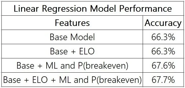
The model that produced the most accurate results included both the breakeven win probabilities and each team’s ELO. While it doesn’t beat the Vegas prediction, this model got extremely close. The most significant features in this model were the team WL% and the breakeven win probabilities by far. Interesting, this model generated $0 in profit, as the predictions made were always too close to the Vegas predictions, and so no bets were ever placed.
results
We also decided to perform one last apples-to-apple test, where we fed the same set of features into each model to gauge the relative performance of each model. We also create a cumulative profit graph for each model, which shows not just how our models do at the end of season, but if we could even afford to make it to end anyways (If we lose $100,000 before we make it all back, perhaps we wouldn’t remain so confident). Results are summarized in the table below, with cumulative profit graphs following.


You can click on a profitability graph to enlarge the view. In the end, the ultimate question is whether we can consider the outcome a success. Currently, that answer is no - none of our models outperformed Vegas, and even the most profitable of our models has a p-value of 0.192 associated with it against completely random predictions. As a result, it’s hard to conclusively say that our models are working well enough for us to quit our jobs.
discussion and future work
Many options are available toward furthering our work. For one, we could try calculating season averages for features we ignored (e.g. rebounds, assists, shooting percentages), right up to that game in the season. Other features we might want to explore include coaching staff, player injuries, and matching up offensive and defensive players (as discussed in the k-NN section). We could also look into different preprocessing strategies for the data we’re currently using. Moving onto the modeling stage of the process, perhaps we could consider different modeling approaches: for example, Random Forests or Naive Bayes. Additionally, perhaps an ensembling of all of the models we’ve built could be helpful.
We could also expand the scope of our work to predict preseason and playoff games, or to predict different target variables (e.g. the point spread, the total number of points scored in a match, or any other betting markets available). Finally, we could look into alternative betting strategies (e.g. the Kelly criterion).
[1] If the moneyline is negative (usually in the case of a favored team), then the breakeven probability is ML / (100 + ML). If the moneyline is positive (usually for the underdog), then the breakeven probability is 100 / (ML + 100). Usually, adding up the breakeven probabilities for the home and away team was higher than 100%, which reflects one method by which Vegas profits.
[2] We're assuming no transaction fees, which isn't realistic, but since the moneylines are already set such that Vegas has an edge, we're still not playing on even ground.